Multivariate Gaussian Distribution in Python
- Normal Distribution - {:.} Code Example
- Standard Normal Distribution - {:.} Z-Score Code - {:.} Standard Normal Distribution Code - {:.} [NOTE] Sampling Distribution of the Mean
- Multivariate Normal Distribution - {:.} 2 dimensional visual example - {:.} 남자 여자의 키 분포 예제
Normal Distribution
사람의 키, 측정치의 오류률, 혈압, 시험성적등등 많은 데이터의 유형이 gaussian distribution(normal distribution)을 따릅니다.
평균값과 분산값만 알고 있다면 central theorem을 통해 분포도를 알 수 있습니다.
데이터가 정규분포를 따를때..
68%는 1 std안에 존재하고, 95%는 2 std안에 존재하며, 99.7%는 3 std안에 존재합니다.
Gaussian distribution의 공식은 다음과 같으며, probability density function으로도 불립니다.
PDF는 어떤 구간[a, b] 안에 확률 변수 X가 포함될 확률을 나타냅니다.
앞의 계수(coefficient) \(\frac{1}{\sqrt{2\pi \sigma^2}}\)는 x에 의존하지 않는 상수로 볼 수 있습니다.
따라서 일종의 normalization factor로 볼 수 있습니다.
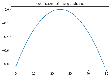
\(-\frac{(x-\mu)^2}{2 \sigma^2}\) 이 부분이 quadratic function (2차함수) of the variable x 입니다.
2차함수의 계수(the coefficient of the quadratic term)는 음수이므로 포물선(parabola)는 downwards입니다.
참고로 downward parabola는 다음과 같이 생겼습니다.
Code Example
from scipy.stats import norm

def normal_distribution(x):
    var = np.var(x)
    mean = np.mean(x)
    r = np.exp(-(x-mean)**2/(2*var))/ (np.sqrt(2 * np.pi * var))
    return r

def example_normal_distributions(mean):
    x = np.linspace(norm.ppf(0.0001), norm.ppf(0.9999), 100) + mean
    my_y = normal_distribution(x)
    scipy_y = norm.pdf(x, loc=mean, scale=np.std(x))

    plt.plot(x, my_y, alpha=0.5, color='blue', label='my normal distribution')
    plt.plot(x, scipy_y, alpha=0.5, color='red', label='scipy normal distribution')
    plt.title(f'mean: {x.mean():3.3}   std: {x.std():3.3}')
    plt.legend()

example_normal_distributions(mean=15)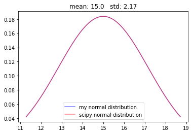
Standard Normal Distribution
Normal distribution을 결정짓는 2가지 요소는 mean 그리고 variance입니다.
Normal distribution과 standard normal distribution의 차이는 바로 standard normal distribution의 경우 mean은 9값을 갖고, variance는 1값을 갖습니다.
(variance에다가 루트를 씌운것이 standard deviation인데.. 결국 \(\sqrt{1} = 1\) 이므로, standard normal distribution은 std = variance = 1을 갖게 됩니다)
\(X\) 라는 값이 특정 mean 과 variance 값을 가진 normal distribution일때, Z-Score를 계산함으로서 standard normal distribution으로 변환해줄 수 있습니다.
Z-Score Code
def z_score(X):
    return (X - np.mean(X))/np.std(X)

x = np.linspace(norm.ppf(0.0001), norm.ppf(0.9999), 1000)
z = z_score(x)

# 다음은 결과
x mean: 1.42108547152e-14
x std : 2.14932341883
x variance: 4.61959115873
z score mean: 0.0
z score std : 1.0
z score variance: 1.0
Standard Normal Distribution Code
def example_normal_distributions(mean):
    x = np.linspace(norm.ppf(0.0001), norm.ppf(0.9999), 1000) + mean
    std = np.std(x)

    general_norm_data1 = norm.pdf(x, loc=mean, scale=std)
    general_norm_data2 = normal_distribution(x)

    std_norm_data1 = norm.pdf(z_score(x), loc=0, scale=1)
    std_norm_data2 = normal_distribution(z_score(x))
    # ... 생략

    plots[0].plot(x, general_norm_data1, alpha=0.5, color='blue', label='scipy normal dist')
    plots[0].plot(x, general_norm_data2, alpha=0.5, color='red', label='my normal dist')
    plots[1].plot(z_score(x), std_norm_data1, alpha=0.5, color='blue', label='z-score > scipy norm dist')
    plots[1].plot(z_score(x), std_norm_data2, alpha=0.5, color='red', label='z-score > my norm dist')
    # ... 생략
example_normal_distributions(mean=15)
결과 값
[random variable X]
  mean    : 15.0
  std     : 2.14932341883
  variance: 4.61959115873

[Z-score X]
  mean    : 0.0
  std     : 1.0
  variance: 1.0

MSE General  Normal Distribution: 0.0
MSE Standard Normal Distribution: 0.0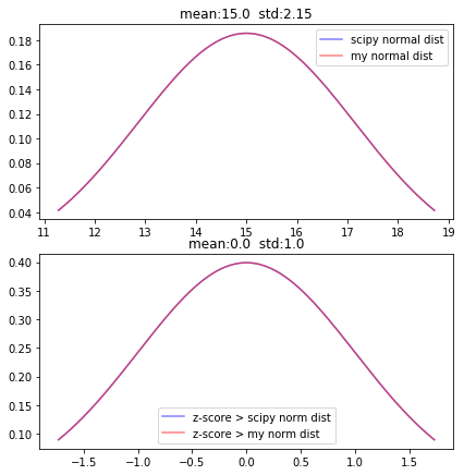
[NOTE] Sampling Distribution of the Mean
어떤 분포이든지간에 표본의 평균(sample mean)은 normal distribution을 따릅니다.
예를 들어서 2000명의 학생들이 종이 쪽이에 0에서 100사이의 숫자를 적은뒤 상자안에 넣습니다.
수학선생님이 랜덤으로 30개의 종이쪽지를 꺼내서 평균을 냅니다. 만약 선생님이 이 작업을 여러번 할 경우
표본의 평균은 확률분포는 정규분포를 갖게 됩니다.
아래는 코드로 설명한 것입니다.
def test_sample_mean_is_normal_distribution(n=1000):
    X = np.random.randint(0, 100, size=2000)
    samples = np.zeros(n, dtype='float32')
    for i in range(n):
        idx = np.random.randint(0, 100, size=30)
        samples[i] = X[idx].mean()
    return samples

sample_means = test_sample_mean_is_normal_distribution(n=50000)
plt.hist(sample_means, bins=100)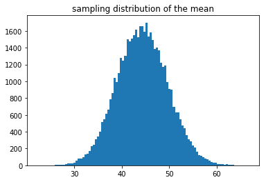
Multivariate Normal Distribution
한국어로 다변수 또는 다변량 정규분포라고 하며, 다차원의 공간에 확장한 분포입니다.
Probability density function은 다음과 같이 정의 됩니다.
- \(k\) : Component distribution의 갯수
- \(\| \Sigma \|\) : determinant of \(\Sigma\) 를 가르킵니다. 즉.. \(\det(\Sigma)\) 로 표현될수 있습니다.
- \((\mathbf{x} - \mathbf{\mu})^T \Sigma^{-1} (\mathbf{x} - \mathbf{\mu})\) : Mahalanobis distance
- \(\mu \in \mathbb{R}^n\) 이므로 각 dimension마다의 평균값을 갖은 vector라고 생각하면 됩니다.
- \(\Sigma \in \mathbb{R}^{n*n}\) 이므로 covariance matrix는 (n, n) shape의 matrix라고 생각하면 됩니다.
Numpy의 multivariate_normal 사용시 1차원의 vector로 사용도 가능하고, 상수도 됩니다.
2 dimensional visual example
def example_multivariate_normal_distribution2():
    x, y = np.mgrid[-1:1:0.01, -1:1:.01]
    pos = np.dstack((x, y))

    rv1 = multivariate_normal(mean=[0, 0], cov=[[0.1, 0],[0, 0.1]])
    rv2 = multivariate_normal(mean=[0, 0], cov=[[1, 0],[0, 1]])
    rv3 = multivariate_normal(mean=[0.5, -1], cov=[[1, 0],[0, 1]])

    rv4 = multivariate_normal(mean=[0, 0], cov=[[1, 0],[0, 1]])
    rv5 = multivariate_normal(mean=[0, 0], cov=[[1, 0.5],[0.5, 1]])
    rv6 = multivariate_normal(mean=[0, 0], cov=[[1, 0.9],[0.9, 1]])

    rv7 = multivariate_normal(mean=[0, 0], cov=[[1, 0],[0, 1]])
    rv8 = multivariate_normal(mean=[0, 0], cov=[[1, -0.5],[-0.5, 1]])
    rv9 = multivariate_normal(mean=[0, 0], cov=[[1, -0.9],[-0.9, 1]])

    fig, subplots = plt.subplots(3, 3)
    fig.set_figwidth(14)
    fig.set_figheight(14)
    subplots = subplots.reshape(-1)

    subplots[0].contourf(x, y, rv1.pdf(pos), cmap='magma')
    subplots[1].contourf(x, y, rv2.pdf(pos), cmap='magma')
    # 생략...

    subplots[0].set_title('mean=0 cov=[.1, 0]')
    subplots[1].set_title('mean=0 cov=[1, 0]')
    # 생략...

example_multivariate_normal_distribution2()
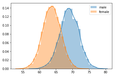
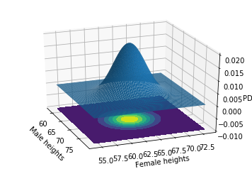
남자 여자의 키 분포 예제
# Get Data
data = pd.read_csv('dataset/gender-height-weight.csv', usecols=(0, 1, 2))
# data = pd.get_dummies(data, columns=['Gender'], prefix='', prefix_sep='')

data = np.dstack([data[data['Gender'] == 'Male']['Height'],
                  data[data['Gender'] == 'Female']['Height']])[0]


# Mean vector and covariance matrix
cov = np.cov(data[:, 0], data[:, 1])
mean = data.mean(axis=0)

# 2-dimensional distribution
x_min, x_max = data[:, 0].min(), data[:, 0].max()
y_min, y_max = data[:, 1].min(), data[:, 1].max()
x, y = np.mgrid[x_min:x_max:0.1, y_min:y_max:.1]
pos = np.dstack((x, y))

# Calculate Multivariate gausian distributions
z = multivariate_normal.pdf(pos, mean=mean, cov=cov)

# Visualization
print(f'[Male  ] x_min: {x_min:<6.3} \tx_max:{x_max:<6.3}')
print(f'[Female] y_min: {y_min:<6.3} \ty_max:{y_max:<6.3}')
print('mean:', mean)

# First Plot
sbn.distplot(data[:, 0], bins=25, label='male')
sbn.distplot(data[:, 1], bins=25, label='female')
plt.legend()

# Second 3d Plot
fig = plt.figure()
ax = fig.gca(projection='3d')
ax.plot_surface(x, y, z, rstride=3, cstride=3, linewidth=1, antialiased=True)
ax.contourf(x, y, z, zdir='z', offset=-0.01)

# Adjust the limits, ticks and view angle
ax.set_zlim(-0.01,0.02)
ax.view_init(27, -21)
ax.set_xlabel('Male heights')
ax.set_ylabel('Female heights')
ax.set_zlabel('PDF')
결과값 입니다.
[Male  ] x_min: 58.4   	x_max:79.0
[Female] y_min: 54.3   	y_max:73.4
mean: [ 69.02634591  63.7087736 ]