TF-IDF
1. TF-IDF
1.1 TF
\[TF(t, d) = \frac{\text{t의 갯수 in d}}{\text{단어의 갯수 in d}}\]- TF는 기본적으로 문서 하나에서의 특정 단어 갯수를 의미 한다.
- stopwords 가 높은 값으로 나옴
- t : term (word)
- d : document (문서 하나를 의미)
- corpus: set of documents (전체 문서들을 의미)
TF만으로 단어의 중요성을 수치로 나타내면 좋겠지만, 문제는 is, are, the 같은 stopwords 가 높은 값을 가지게 됩니다.
보완할 필요가 있습니다.
1.2 DF
\[DF = \text{t를 포함하고 있는 document의 갯수}\]예를 들어, “사과”라는 단어가 document 1 에서 50번 나오고, document 2에서 100번, 그리고 document 3에서 0번 나온다면..
DF의 값은 2 입니다. 왜냐하면 “사과”를 포함하고 있는 문서의 갯수는 2개 이기 때문입니다.
1.3 IDF
\[\begin{align} \text{IDF (vanila)} &= \log\left( \frac{N}{df} \right) \\ \text{IDF (smooth)} &= \log\left( \frac{N}{df} \right) +1 \\ \text{IDF (another smooth)} &= \log\left( \frac{N}{df + 1} \right) +1 \\ \end{align}\]- 주 목적은 TF에서 높에 나온 stopwords들을 값을 낮추도록 weight를 줌
- stopwods에 대한 값은 매우 낮게 나옴
- log 를 사용하는 이유는 N값이 높아질수록 값이 커지는 문제를 해결하기 위해서
1.4 TF-IDF
\[\text{TF-IDF}(t, d) = TF \times IDF\]최종적으로 TF 그리고 IDF 를 서로 곱해주면 TF-IDF 값이 나옵니다.
* SKLearn에서 구현한 것을 똑같이 해보려고 하였으나, 공식이 좀 다른듯 함.
2. SKLearn
2.1 Data
corpus = [
    'This is the first document. is this first one? this is the first one',
    'This document is the second document. the document!',
    'this is document. is this the second document?',
    'Is this the robot document?',
    'this is the document. this is the first one document.',
    'this this this the the the first is is is document document',
]
2.2 Code
import seaborn as sns
from sklearn.feature_extraction.text import TfidfVectorizer
cm = sns.light_palette('red', as_cmap=True)
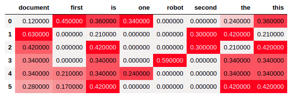
vectorizer = TfidfVectorizer()
tfidf_mtx = vectorizer.fit_transform(corpus).toarray()
tfidf_df = pd.DataFrame(tfidf_mtx.round(2),
columns=vectorizer.get_feature_names())
tfidf_df.style.background_gradient(cmap=cm)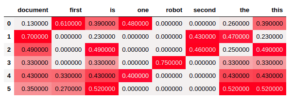
3. Numpy
3.1 Counter
from sklearn.feature_extraction.text import CountVectorizer

cvec = CountVectorizer()
cnt_mtx = cvec.fit_transform(corpus).toarray()
columns = cvec.get_feature_names()
counter_df = pd.DataFrame(cnt_mtx,
                          columns=columns)
counter_df.style.background_gradient(cmap=cm)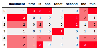
3.2 TF
빈번하게 나오는 단어들은 값이 높게 나옵니다.
실제로 is, this, document 같이 많이 나온 단어일수록, TF의 평균값은 높게 나옵니다.
# TF
tf = (cnt_mtx/cnt_mtx.sum(axis=1)[:, None])

# Visualization
_df = pd.DataFrame(tf.round(2), columns=columns)

display(_df.style.background_gradient(cmap=cm))
_df = pd.DataFrame({'sum': counter_df.sum(),
                    'mean': _df.mean(),
                    'max': _df.max(),
                    'min': _df.min()})
_df.sort_values('sum', ascending=False)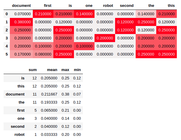
3.3 DF
해당 단어를 포함하고 있는 document의 갯수 입니다.
# DF
df = cnt_mtx.astype(bool).sum(axis=0).astype(float)
display(pd.DataFrame([df], columns=columns))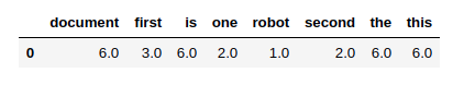
3.4 IDF
IDF에서는 TF와는 반대로 stopwords (is, this, document, the) 같은 단어들의 IDF값이 더 작습니다.
즉 rare 한 단어들일수록 IDF값은 높아집니다.
# IDF
n_d, _ = cnt_mtx.shape
idf = np.log(n_d/df + 1) + 1

display(pd.DataFrame([idf], columns=columns))

# Visualization
_df = pd.DataFrame({'sum': counter_df.sum(),
                    'idf': idf})
_df.sort_values('sum', ascending=False)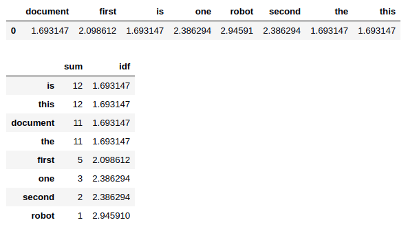
3.5 TF-IDF
최종적으로 tf * idf 를 합니다.
tfidf_ = (tf * idf)

_df = pd.DataFrame(tfidf_.round(2), columns=columns)
_df.style.background_gradient(cmap=cm)