Multiple Linear Regression
- Formula
- Predicting Medical Expenses - {:.} Correlation Matrix - {:.} Model Performance
- Matrix Inverse

Formula
일단 Multiple Regression은 다음과 같이 생겼습니다.
- \(\alpha\): y-intercept
- \(\epsilon\): 그리스어로 epsilon이며, Error를 나타냅니다.
\(\beta_{1}\), \(\beta_{2}\) 처럼 Coefficients들이 각각의 features들이 붙어있는데, 이는 각각의 feature(x값)들이 따로따로 y값에 대해서 estimated effect를 갖기 위함입니다. (즉 각각의 feature들마다 slope이 있다고 생각하면 됨)
이때 y-intercept값은 다른 Regression Parameters들과 별 차이가 없기 때문에 다음과 같이 \(x_{0} = 1\) 로 잡아서 다음과 같이 쓸수 있습니다. (\(\beta_{0}\)은 beta-naught라고 발음합니다.) -> 계산을 편하게 하기 위함
\[y = \beta_{0}x_{0} + \beta_{1}x_{1} + \beta_{2}x_{2} + \ ... \ + + \beta_{i}x_{i} + \epsilon\]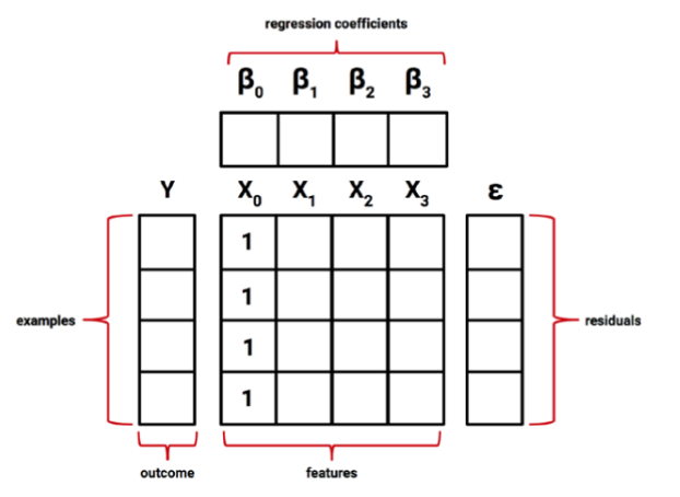
궁극적인 목표는 Sum of the squared errors를 구했을때 error가 가장적은 \(\beta\) (The vector of regression coefficients)값을 찾는 것입니다.
\[\hat{\beta} = (X^{T}X)^{-1}X^{T}Y\]- T 는 Transpose를 뜻하고, negative exponent는 matrix inverse를 뜻합니다.
R
reg <- function(y, x){
  x <- as.matrix(x)
  x <- cbind(Intercept=1, x) # Intercept 라는 column을 추가시킵니다. 안의 데이터는 모두 1값
  b <- solve(t(x) %*% x) %*% t(x) %*% y # solve 는 inverse of a matrix를 취합니다.
  colnames(b) <- 'estimate'
  print(b)
}

reg(y=challenger$distress_ct, x=challenger[2:4])
                         estimate
Intercept             3.527093383
temperature          -0.051385940
field_check_pressure  0.001757009
flight_num            0.014292843
Python
import numpy as np
from numpy.linalg import inv

challenger = np.genfromtxt('challenger.csv', delimiter=',', skip_header=True)

def reg(x, y):
    x = np.c_[np.ones(len(x)), x]
    b = inv(np.dot(x.T, x))
    b = np.dot(np.dot(b, x.T), y)
    return b[0], b[1:]

y_intercept, coefficients = reg(y=challenger[:, 0], x=challenger[:, 1:4])
# y_intercept:  3.52709338331
# coefficients: [-0.05138594  0.00175701  0.01429284]
Predicting Medical Expenses
Correlation Matrix
R
cor(insurance[c('age', 'bmi', 'children', 'expenses')])
               age        bmi   children   expenses
age      1.0000000 0.10934101 0.04246900 0.29900819
bmi      0.1093410 1.00000000 0.01264471 0.19857626
children 0.0424690 0.01264471 1.00000000 0.06799823
expenses 0.2990082 0.19857626 0.06799823 1.00000000
Python Pandas
data = pd.read_csv('../data/multiple-linear-regression/insurance.csv')
data['smoker'] = data['smoker'].apply({'yes': 1, 'no': 0}.get)
data['male'] = data['sex'] == 'male'
data['female'] = data['sex'] == 'female'
data = data[['age', 'sex', 'bmi', 'children', 'smoker', 'region', 'male', 'female', 'expenses']]

data.corr()
               age       bmi  children    smoker      male    female  expenses
age       1.000000  0.109341  0.042469 -0.025019 -0.020856  0.020856  0.299008
bmi       0.109341  1.000000  0.012645  0.003968  0.046380 -0.046380  0.198576
children  0.042469  0.012645  1.000000  0.007673  0.017163 -0.017163  0.067998
smoker   -0.025019  0.003968  0.007673  1.000000  0.076185 -0.076185  0.787251
male     -0.020856  0.046380  0.017163  0.076185  1.000000 -1.000000  0.057292
female    0.020856 -0.046380 -0.017163 -0.076185 -1.000000  1.000000 -0.057292
expenses  0.299008  0.198576  0.067998  0.787251  0.057292 -0.057292  1.000000
from pandas.tools.plotting import scatter_matrix
scatter_matrix(data, figsize=(10, 10))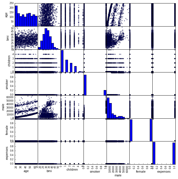
- age ~ bmi: 0.109341 => Weak Positive Correlation을 갖고 있다.
즉 age가 들수록 body mess 또한 조금씩 조금씩 증가한다. - age ~ expenses: 0.299008 그리고 bmi ~ expenses: 0.198576
즉 age, bmi등이 높아질수록, 의료 비용이 많이 들어감을 알 수 있다.
Model Performance
R
ins_model = lm(expenses~age+children+bmi+sex+smoker+region, data=insurance)
Coefficients:
    (Intercept)              age         children              bmi          sexmale        smokeryes
       -11941.6            256.8            475.7            339.3           -131.4          23847.5
regionnorthwest  regionsoutheast  regionsouthwest
-352.8 -1035.6 -959.3 summary(ins_model)
Residuals:
Min 1Q Median 3Q Max
-11302.7 -2850.9 -979.6 1383.9 29981.7
Coefficients:
Estimate Std. Error t value Pr(>|t|)
(Intercept) -11941.6 987.8 -12.089 < 2e-16 ***
age 256.8 11.9 21.586 < 2e-16 ***
children 475.7 137.8 3.452 0.000574 ***
bmi 339.3 28.6 11.864 < 2e-16 ***
sexmale -131.3 332.9 -0.395 0.693255
smokeryes 23847.5 413.1 57.723 < 2e-16 ***
regionnorthwest -352.8 476.3 -0.741 0.458976
regionsoutheast -1035.6 478.7 -2.163 0.030685 *
regionsouthwest -959.3 477.9 -2.007 0.044921 *
---
Signif. codes: 0 ‘***’ 0.001 ‘**’ 0.01 ‘*’ 0.05 ‘.’ 0.1 ‘ ’ 1
Residual standard error: 6062 on 1329 degrees of freedom
Multiple R-squared: 0.7509, Adjusted R-squared: 0.7494
F-statistic: 500.9 on 8 and 1329 DF, p-value: < 2.2e-16- p-value
Python Pandas
from pandas.stats.api import ols
ols(y=data['expenses'], x=data[['age', 'bmi', 'children', 'smoker', 'sex']])

-------------------------Summary of Regression Analysis-------------------------

Formula: Y ~ <age> + <bmi> + <children> + <smoker> + <sex> + <intercept>

Number of Observations:         1338
Number of Degrees of Freedom:   6

R-squared:         0.7497
Adj R-squared:     0.7488

Rmse:           6069.5393

F-stat (5, 1332):   798.0838, p-value:     0.0000

Degrees of Freedom: model 5, resid 1332

-----------------------Summary of Estimated Coefficients------------------------
      Variable       Coef    Std Err     t-stat    p-value    CI 2.5%   CI 97.5%
--------------------------------------------------------------------------------
           age   257.7192    11.9036      21.65     0.0000   234.3881   281.0503
           bmi   322.4516    27.4171      11.76     0.0000   268.7141   376.1891
      children   474.6020   137.8515       3.44     0.0006   204.4132   744.7909
        smoker 23822.3127   412.5110      57.75     0.0000 23013.7911 24630.8342
           sex   128.6813   333.3502       0.39     0.6995  -524.6852   782.0477
--------------------------------------------------------------------------------
     intercept -12312.5200  1084.2038     -11.36     0.0000 -14437.5594 -10187.4805
---------------------------------End of Summary---------------------------------
Matrix Inverse
\[A A^{-1} = I\]- I 는 Identity Matrix 입니다.
import numpy as np
from numpy.linalg import inv

a = np.array([[4., 7.], [2., 6.]])
# array([[ 4.,  7.],
#        [ 2.,  6.]])

inv(a)
# array([[ 0.6, -0.7],
#        [-0.2,  0.4]])

np.dot(a, inv(a))
# array([[ 1.,  0.],
#        [ 0.,  1.]])