Jupyter & Perceptron
- Installation - {:.} Example - {:.} Installing Jupyter - {:.} 한글 설정 - {:.} Increase Jupyter Width Window Size
- Perceptron - {:.} Training Machine Learning Algorithms - {:.} Net Input - {:.} Activation Function - {:.} Perceptron Learning Steps - {:.} Cost Function (Sum of squared Errors) - {:.} Calculate Gradient with regard to weights - {:.} Calculate Gradient with regard to bias - {:.} Update Weights
- Iris Data
- to Python

Installation
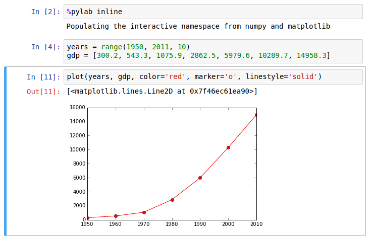
Example
예제는 Python Matplotlib의 plot을 보는 예제
Installing Jupyter
쥬피터는 Ipython Notebook에서 더 발전된 버젼으로 Python, R, Scala등의 데이터 분석에 쓰이는 언어들을 선택해서 웹애플리케이션으로 사용이 가능하게 해줍니다.
sudo pip install jupyter
jupyter notebook
한글 설정
문서의 가장 윗쪽에 다음과 같이 설정합니다.
#-*- coding:utf-8 -*-
%pylab inline
matplotlib.rc('font', family='NanumGothic')
만약 내가 갖고 있는 모든 폰트들을 열고 싶다면..
import matplotlib.font_manager
print [f.name for f in matplotlib.font_manager.fontManager.ttflist]
Increase Jupyter Width Window Size
~/.jupyter/custom/custom.css 에다가 다음을 내용을 넣습니다.
/* Make the notebook cells take almost all available width */
.container {
    width: 99% !important;
}

/* Prevent the edit cell highlight box from getting clipped;
 * important so that it also works when cell is in edit mode*/
div.cell.selected {
    border-left-width: 1px !important;
}
Perceptron
Training Machine Learning Algorithms
Perceptron을 이용해서 Binary Classification을 할 수 있습니다. (0 과 1처럼 2개의 분류로 나뉘는 것)
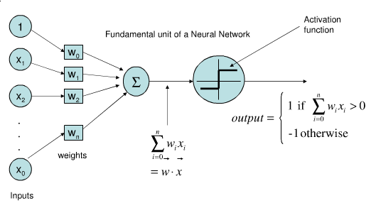
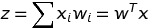
Net Input
- x는 input values로서 1차원 vector입니다.
- w는 그에 일치하는 weight vector입니다.
- z는 net input 입니다. (위의 사진에서 inputs -> weights -> sigma 를 지난 부분)
- Matrix 의 transpose를 사용해서 sum(sigma)를 대체할수 있습니다.
Activation Function
Activation Function  의 output이
Threshold
의 output이
Threshold 보다 더 크다면 1로 예측할수 있고, 아니라면 -1로 예측 할 수 있습니다.
Perceptron Learning Steps
초기 MCP neuron 과 Rosenblatt’s thresholded perceptron model은 매우 간단합니다.
- weigts 는 0또는 작은 랜덤값들로 초기화
- 각각의 training sample
 은 먼저 예측값
  을 알아낸 후, weights를 업데이트 해줍니다.
weights에 대한 업데이트 공식은 다음과 같습니다.
 의 값은 Perceptron Learning Rule에 의해서 알아낼수 있습니다.
- 궁극적으로 이 y값과 일치하면 0이 되기 때문에 weight에 학습 조정은 없습니다.
 Eta는 Learning Rate로서 0~1사이의 값을 갖습니다.
- 만약 예측값 에 오류가 있다면, 는
음수 또는 양수로 떨어지게 됩니다.
- 의 크기는 x의 값에 비례해서 달라지게 됩니다.
Cost Function (Sum of squared Errors)
먼저 Object function $ J(w) $ (Sum of squared Errors - SSE) 를 정의합니다.
이때 $ \phi(z^{(i)}) $ 는 Identity activation function 입니다.
Calculate Gradient with regard to weights
\[\begin{align} \frac{\partial J}{\partial w_j} &= \frac{\partial}{\partial w_j} \frac{1}{N} \sum_i \left(y^{(i)} - \phi(z^{(i)}) \right)^2 \\ &= \frac{2}{N} \sum_i \left( y^{(i)} - \phi(z^{(i)}) \right) \frac{\partial}{\partial w_j} \left(y^{(i)} - \phi(z^{(i)}) \right) \\ &= \frac{2}{N} \sum_i \left( y^{(i)} - \phi(z^{(i)}) \right) \frac{\partial}{\partial w_j} \left[ y^{(i)} - \sum_k \left( w^{(i)}_k x^{(i)}_k + b^{i} \right) \right] \\ &= \frac{2}{N} \sum_i \left( y^{(i)} - \phi(z^{(i)}) \right)(0 - (1 \cdot x^{(i)}_j + 0 ) ) \\ &= - \frac{2}{N} \sum_i \left( y^{(i)} - \phi(z^{(i)}) \right) \odot x^{(i)}_j \end{align}\]Calculate Gradient with regard to bias
\[\begin{align} \frac{\partial J}{\partial b_j} &= \frac{\partial}{\partial b_j} \frac{1}{N} \sum_i \left(y^{(i)} - \phi(z^{(i)}) \right)^2 \\ &= \frac{2}{N} \sum_i \left( y^{(i)} - \phi(z^{(i)}) \right) \frac{\partial}{\partial b_j} \left(y^{(i)} - \phi(z^{(i)}) \right) \\ &= \frac{2}{N} \sum_i \left( y^{(i)} - \phi(z^{(i)}) \right) \frac{\partial}{\partial b_j} \left[ y^{(i)} - \sum_k \left( w^{(i)}_k x^{(i)}_k + b^{i} \right) \right] \\ &= \frac{2}{N} \sum_i \left( y^{(i)} - \phi(z^{(i)}) \right)(0 - (0 + 1 ) ) \\ &= - \frac{2}{N} \sum_i \left( y^{(i)} - \phi(z^{(i)}) \right) \end{align}\]Update Weights
\[\begin{align} \Delta w &= - \eta \nabla J(w) \\ w &= w + \Delta w \end{align}\]Iris Data
1930sus 식물학자 Edgar Anderson은 붓꾳(Iris)에 대한 데이터를 수집했습니다.
그는 그 데이터가 현대 머신러닝뿐만 아니라 데이터 싸이언스의 기초 과정이 되리라고는 전혀 예상치 못했겠죠.
었쨌든 iris 데이터는 수많은 머신러닝의 테스트 케이스또는 기초 연구용으로 사용되는 아주 중요한 데이터입니다.
데이터는 다음과 같이 구성되어 있습니다.
- Sepal.Length
- Sepal.Width
- Petal.Length
- Petal.Width
- Species
df = pd.read_csv('iris.csv', header=None)
setosa = df[df[4] == 'Iris-setosa']
versicolor = df[df[4] == 'Iris-versicolor']
virginica = df[df[4] == 'Iris-virginica']

a, b = 0, 3
plt.scatter(setosa[a], setosa[b], color='red', marker='o', label='setosa')
plt.scatter(versicolor[a], versicolor[b], color='blue', marker='x', label='versicolor')

plt.xlabel('Petal Length')
plt.ylabel('Sepal Length')
plt.legend(loc='upper left')
plt.grid()
plt.show()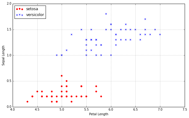
to Python
Perceptron
import numpy as np

class Perceptron(object):

    def __init__(self, learning_rate=0.02):
        self.w = np.random.randn(2 + 1)
        self.eta = learning_rate

    def predict(self, xdata):
        phi = self.w[1:].dot(xdata.T) + self.w[0]
        net = np.where(phi > 0, 1, -1)
        return net

    def relu(self, net):
        return np.maximum(net, 0)

    def train(self, x_trains, y_trains, n_episode=10):
        costs = []

        for self.step in range(n_episode):
            cost = 0

            # Shuffle
            rands = np.random.permutation(len(x_trains))
            x_trains = x_trains[rands]
            y_trains = y_trains[rands]

            for xi, yi in zip(x_trains, y_trains):
                output = self.predict(xi)

                update = self.eta * np.sum(yi - output)
                self.w[1:] += update * xi
                self.w[0] += update

                cost += np.sum((yi - output)**2)/2.

            costs.append( cost/len(x_trains))
        return costs


    def save(self):
        np.save(open('iris.weights', 'wb'), perceptron.w)

    def load(self):
        self.w = np.load(open('iris.weights', 'rb'))

    def cost(self, predicted_ys, ys):
        ys - predicted_ys
y = df.iloc[0:100, 4].values
y = np.where(y == 'Iris-setosa', -1, 1)
X = df.iloc[0:100, [0, 3]].values
perceptron = Perceptron()
costs = perceptron.train(X, Y)
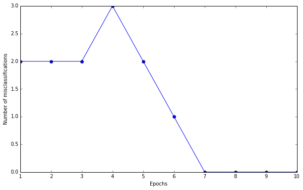
plt.plot(range(1, len(ppn._errors) + 1), ppn._errors, marker='o')
plt.xlabel('Epochs')
plt.ylabel('Number of misclassifications')
plt.show()Perceptron Machine Learning 을 이용해서 기계에 학습을 시킨후 에러률을 출력해봤습니다.
처음에 에러가 2~3개정도씩 나오다가.. 대략 7번이후부터는 정확하게 Classification을 하는 것을 볼수 있습니다.