Adam (Adaptive Moment Estimation)

ADAM: A METHOD FOR STOCHASTIC OPTIMIZATION
An overview of gradient descent optimization algorithms
Deep Learning 301page - Ian Goodfellow, Yoshua Bengio, and Aaron Courville 참고

Pros

RMSProp 또는 AdaDelta처럼 exponentially decaying average of past squared gradients \(v_t\) 값을 갖고 있으며 또한,
Adam은 Momentum처럼 exponentially decaying average of past gradients \(m_t\)값을 갖고 있습니다.
Data 그리고 parameters(weights)가 larse size에 적합하다
non-stationary, noisy, sparse 문제에 강하다

Algorithm

Require
1. Step Size \(\alpha\) (suggested default: 0.001)
2. Exponential decay rates for the moment estimates: \(\beta_1 \beta_2 \in [0, 1)\)
3. Epsilon \(\epsilon\) (보통 \(10^{-8}\))
Initialization
1. Parameters (weights) \(\theta\)
2. \(m_0 = 0\) (1st moment vector - exponentially decaying average of past gradients)
3. \(v_0 = 0\) (2st moment vector - exponentially decaying average of past squared gradients)
  여기서 squared gradients란 \(g_t \odot g_t\)
4. Initialize Timestep \(t = 0\)
Pseudo Code
- while \(\theta_t\) not converged do:
  1. Sample a minibatch
  2. t = t + 1
  3. Compute Gradient
    \(g_t = \frac{1}{N} \nabla_{\theta} \sum_i L\left( f(x^{(i)}; \theta), y^{(i)} \right)\)
  4. Update biased first moment estimate:
    \(m_t = \beta_1 \cdot m_{t-1} + (1-\beta_1) \odot g_t\)
  5. Update biased second raw moment estimate:
    \(v_t = \beta_2 \cdot v_{t-1} + (1-\beta_2) \odot g^2_t\)
  6. Correct bias in first moment:
    \(\hat{m}_t = \frac{m_t}{1-\beta^t_1}\)
  7. Correct bias in second moment:
    \(\hat{v}_t = \frac{v_t}{1-\beta^t_2}\)
  8. Compute Update:
    \(\Delta \theta_t = \alpha \frac{ \hat{m}_t}{\sqrt{\hat{v}_t} + \epsilon}\)
  9. Update weights:
    \(\theta_t = \theta_{t-1} - \Delta \theta_t\)
- end while

Explain Algorithm

Exponential moving averages

알고리즘은 exponential moving averages of the gradient \(m_t\), 그리고 exponential moviing averages of the squared gradient \(v_t\) 값을 hyper-parameters 인 \(\beta_1, \beta_2 \in [0, 1)\)의 값에 따라 decay rate를 조정함으로서 컨트롤합니다. 즉 \(\beta_1, \beta_2\)의 값이 1에 가까울수록 decay rate는 작아지며, 이전 \(t-1\)의 영향력이 커지게 됩니다. 예를 들어서..

\[m_t = \beta_1 \cdot m_{t-1} + (1-\beta_1) \odot g_t\]

위의 공식에서 \(\beta_1 = 0.9\) 라면 다음과 같이 됩니다.

\[0.9 \cdot m_{t-1} + 0.1 \odot g_t\]

gradient \(g_t\) 의 반영이 0.1 밖에 되지 않으며, 초기 \(m\)값 자체가 0값으로 초기화 되어 있기 때문에, 0값으로 bias할 가능성이 큽니다.
심지어 \(\beta_1 = 1\) 이면 학습이 되지 않습니다.

Correct bias

Why is it important to include a bias correction term for the Adam optimizer for Deep Learning?

위에서 설명한대로 초기 moving averages의 값들이 0으로 설정되며, 특히 decay rate 가 작을수록 (\(\beta_1, \beta_2\)의 값이 1에 가까움) moment estimates의 값이 0으로 bias될 수 있습니다. 하지만 Adam optimizer는 bias부분을 교정하는 부분을 갖고 있습니다. 예를들어 만약 recursive update를 unfold하면 다음과 같이 됩니다. 즉 \(\hat{m}_t\) 는 weighted average of the gradients 입니다.

\[\hat{m}_t=\frac{\beta^{t-1}g_1+\beta^{t-2}g_2+...+g_t}{\beta^{t-1}+\beta^{t-2}+...+1}\]

\(m_1\leftarrow g_1\)
while not converge do:
\(\qquad m_t\leftarrow \beta m_t + g_t\) (weighted sum)
\(\qquad \hat{m}_t\leftarrow \dfrac{(1-\beta)m_t}{1-\beta^t}\) (weighted average)

즉 weighted sum을 바로 update해주지 않고, 평균값으로 적용해주기 때문에 \(\beta_1, \beta_2\)에 대한 영향력이 적어지게 됩니다.

Correct Bias

\(v_t\) 의 값을 reculsive 하게 unfold시키면 다음과 같습니다.
처음 \(\beta_2 v_0\) 이 없어진 이유는 v_0값이 초기에 0으로 세팅되어 있기때문에 그냥 사라짐 ..

\[v_t = \beta_2(1-\beta_2)\odot g^2_{t-1} + \beta_2(1-\beta_2)\odot g^2_{t-2} + \beta_2(1-\beta_2)\odot g^2_{t-3} + ...\]

즉 다음과 같이 표현될수 있습니다.
여기서 \(g^2 = g \odot g\) 과 같습니다.

\[v_t = (1-\beta_2) \sum^t_{i=1} \beta^{t-i}_2 \cdot g^2_i\]

아래는 정말 같은 코드로 돌려봤습니다.

def v1(beta2, t, g):
    V = 0
    for i in range(t):
        V = beta2 * V + (1-beta2) * g**2
    return V

def v2(beta2, t, g):
    return (1 - beta2) * np.sum([beta2**i * g**2 for i in range(t)])

print(v1(0.9, 10, 0.1))
print(v2(0.9, 10, 0.1))

\(\hat{v}_t\)를 recursive하게 돌리면 다음과 같습니다.

\[\frac{(1-\beta_2) \sum^t_{i=1} \beta^{t-i}_2 \cdot g^2_i }{ \sum^t_{i=1} (1-\beta^i_2)}\] \[\hat{v}_t = \frac{v_t}{1-\beta^t_2}\]

Implementation

Import

%pylab inline
import numpy as np
import pandas as pd

from sklearn.model_selection import  train_test_split
from sklearn.preprocessing import StandardScaler
from sklearn.metrics import accuracy_score
from sklearn.datasets import load_iris

Data

iris = load_iris()

# setosa_x = iris.data[:50]
# setosa_y = iris.target[:50]
# versicolor_x = iris.data[50:100]
# versicolor_y = iris.target[50:100]
# scatter(setosa_x[:, 0], setosa_x[:, 2])
# scatter(versicolor_x[:, 0], versicolor_x[:, 2])

# Extract sepal length, petal length from Setosa and Versicolor
data = iris.data[:100, [0, 2]]

# Standardization
scaler = StandardScaler()
data = scaler.fit_transform(data)


# Split data to test and train data
train_x, test_x, train_y, test_y = train_test_split(data, iris.target[:100], test_size=0.3)

# Plotting data
scatter(data[:50, 0], data[:50, 1], label='Setosa')
scatter(data[50:100, 0], data[50:100, 1], label='Versicolour')
title('Iris Data')
xlabel('sepal length')
ylabel('petal length')
grid()
legend()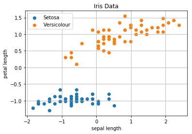

SGD with Adam

w =   np.array([ 0.09370901, -0.24480254, -0.84210235]) # np.random.randn(2 + 1)

def predict(w, x):
    N = len(x)
    yhat = w[1:].dot(x.T) + w[0]
    return yhat

def adam_nn(w, X, Y, eta=0.001, alpha=0.001, beta1=0.9, beta2=0.999, weight_size=2):
    """
    @param eta <float>: learning rate
    @param alpha <float>: Step Size (suggested default is 0.001)
    """
    N = len(X)
    e = 1e-8
    T = 10000
    M = np.zeros(weight_size + 1) # First moment estimate
    V = np.zeros(weight_size + 1) # Second moment estimate

    for t in range(N):
        x = X[t]
        y = Y[t]
        x = x.reshape((-1, 2))
        yhat = predict(w, x)

        # Calculate the gradients
        gradient_w = 2/N*-(y-yhat).dot(x)
        gradient_b = 2/N*-(y-yhat)

        # Update biased first moment estimate
        M[1:] = beta1 * M[1:] + (1-beta1) * gradient_w
        M[0]  = beta1 * M[0]  + (1-beta1) * gradient_b

        # Update biased second raw moment estimate
        V[1:] = beta2 * V[1:] + (1-beta2) * gradient_w**2
        V[0]  = beta2 * V[0]  + (1-beta2) * gradient_b**2

        # Compute bias-corrected first moment estimate
        Mw = M[1:]/(1-beta1**t + e)
        Mb = M[0]/(1-beta1**t + e)

        # Compute bias-corrected second raw moment estimate
        Vw = V[1:]/(1-beta2**t)
        Vb = V[0]/(1-beta2**t)

        # Compute Deltas
        delta_w = alpha * Mw/(np.sqrt(Vw) + e)
        delta_b = alpha * Mb/(np.sqrt(Vb) + e)

#         delta_w = alpha * M[1:]/(np.sqrt(V[1:]) + e)
#         delta_b = alpha * M[0]/(np.sqrt(V[0]) + e)

        w[1:] = w[1:] - delta_w
        w[0] = w[0] - delta_b

    return w


for i in range(30):
    w = adam_nn(w, train_x, train_y)

    # Accuracy Test
    yhats = predict(w, test_x)
    yhats = np.where(yhats >= 0.5, 1, 0)
    accuracy = round(accuracy_score(test_y, yhats), 2)
    print(f'[{i:2}] Accuracy: {accuracy:<4.2}')

[ 0] Accuracy: 0.0
[ 1] Accuracy: 0.0
[ 2] Accuracy: 0.0
[ 3] Accuracy: 0.0
[ 4] Accuracy: 0.0
[ 5] Accuracy: 0.0
[ 6] Accuracy: 0.0
[ 7] Accuracy: 0.13
[ 8] Accuracy: 0.4
[ 9] Accuracy: 0.47
[10] Accuracy: 0.57
[11] Accuracy: 0.63
[12] Accuracy: 0.73
[13] Accuracy: 0.73
[14] Accuracy: 0.8
[15] Accuracy: 0.83
[16] Accuracy: 0.9
[17] Accuracy: 0.93
[18] Accuracy: 0.93
[19] Accuracy: 0.93
[20] Accuracy: 0.93
[21] Accuracy: 0.97
[22] Accuracy: 0.97
[23] Accuracy: 0.97
[24] Accuracy: 0.97
[25] Accuracy: 0.97
[26] Accuracy: 0.97
[27] Accuracy: 0.97
[28] Accuracy: 0.97
[29] Accuracy: 1.0