Cost Functions
- Data
- Mean Squared Error (MSE) - {:.} Partial derivative of the weights - {:.} Partial derivative of the bias variable - {:.} Numpy - {:.} Sklearn - {:.} Visualization
- Mean Absolute Error (MAE) - {:.} Numpy - {:.} Sklearn - {:.} Visualization
- Root Mean Squared Logarithmic Error (RMSLE) - {:.} Numpy - {:.} Visualization
- Binary Cross Entropy (a.k.a Logarithmic Loss) - {:.} Numpy - {:.} Sklearn - {:.} Pytorch - {:.} Visualization
- Cross Entropy - {:.} Partial derivative of the weights - {:.} Partial derivative of the bias - {:.} Numpy - {:.} Pytorch - cross entropy - {:.} Pytorch - Custom Cross Entropy
- Hinge Loss - {:.} Numpy - {:.} Sklearn
- KL-Divergence - {:.} Numpy
- Cosine Proximity - {:.} Numpy - {:.} Visualization
- Poisson - {:.} Numpy

Data
%pylab inline
import numpy as np
from sklearn import metrics
from sklearn.preprocessing import minmax_scale
from scipy import stats
from scipy.spatial.distance import cosine as cosine_distantce

# Pytorch
import torch
from torch import nn
from torch.nn import functional as F
from torch.autograd import Variable

a = np.random.normal(loc=3, size=1000)
b = np.random.normal(loc=3, size=1000)
c = np.random.gumbel(size=1000)
d = np.random.exponential(size=1000)
f = np.random.uniform(size=1000)

hist(a, bins=80, label='nomal a')
hist(b, bins=80, label='normal b')
hist(c, bins=80, label='gumbel c')
hist(d, bins=80, label='exponential d')
hist(f, bins=80, label='uniform f')

grid()
legend()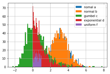
Mean Squared Error (MSE)
regression에서 대체로 많이 사용되는 cost function중의 하나입니다.
단점은 square 를 사용하기 때문에 cost이 지나치게 커져서 unstable 한 모델에 적용시 oscillation 현상이 일어날수 있습니다.
- \(J\) : cost function
- \(\theta\) : parameters (weights)
- N : training data의 갯수
- \(x^{(i)}\) : \(i^{th}\)의 training input vector
- \(y^{(i)}\) : \(i^{th}\)의 class label
- \(h_{\theta} \left( x^{(i)} \right)\) : \(\theta\)를 사용하여 나온 \(i^{th}\) data에 대한 prediction
Partial derivative of the weights
\[\begin{eqnarray} \\ \frac{\partial}{\partial\theta} J(\theta) &=& \frac{\partial}{\partial \theta} \left( \frac{1}{N} \sum^N_{i=1} \left( h_{\theta}(x^{(i)}) - y^{(i)} \right)^2 \right) & [0.1] \\ &=& \frac{2}{N} \sum^{N}_{i=0} \left( h_{\theta} (x^{(i)}) - y^{(i)} \right) \frac{\partial}{\partial \theta} \left( h_{\theta}(x^{(i)}) - y^{(i)} \right) & [0.2] \\ &=& \frac{2}{N} \sum^{N}_{i=0} \left( h_{\theta} (x^{(i)}) - y^{(i)} \right) \frac{\partial}{\partial \theta} \left( \theta^T \cdot x^{(i)} + b - y^{(i)} \right) & [0.3]\\ &=& \frac{2}{N} \sum^{N}_{i=0} \left( h_{\theta} (x^{(i)}) - y^{(i)} \right) \odot x^{(i)} & [0.4]\\ \end{eqnarray}\]0.3 에서 0.4를 넘어갈때 \(\theta\)를 제외하고는 모두 상수이기 때문에 (\(b, x, y\))값 모두 0이 됩니다.
Partial derivative of the bias variable
\[\begin{eqnarray} \\ \frac{\partial}{\partial b} J(\theta) &=& \frac{\partial}{\partial b} \left( \frac{1}{N} \sum^N_{i=1} \left( h_{\theta}(x^{(i)}) - y^{(i)} \right)^2 \right) & [0.1] \\ &=& \frac{2}{N} \sum^{N}_{i=0} \left( h_{\theta} (x^{(i)}) - y^{(i)} \right) \frac{\partial}{\partial b} \left( h_{\theta}(x^{(i)}) - y^{(i)} \right) & [0.2] \\ &=& \frac{2}{N} \sum^{N}_{i=0} \left( h_{\theta} (x^{(i)}) - y^{(i)} \right) \frac{\partial}{\partial b} \left( \theta^T \cdot x^{(i)} + b - y^{(i)} \right) & [0.3]\\ &=& \frac{2}{N} \sum^{N}_{i=0} \left( h_{\theta} (x^{(i)}) - y^{(i)} \right) & [0.4]\\ \end{eqnarray}\]Numpy
>> p = np.array([0.1, 0.1, 0.05, 0.6, 0.3], dtype=np.float32)
>> y = np.array([0, 0, 0, 1, 0], dtype=np.float32)
>>
>> def mean_squared_error(y, p):
>>     return ((y - p)**2).mean()
>>
>> mean_squared_error(y, p)
0.054499995
Sklearn
sklearn에서는 sklearn.metrics.mean_squared_error 함수를 사용하면 됩니다.
>> metrics.mean_squared_error(y, p)
0.054499995
Visualization
>> metrics.mean_squared_error(y, p)
normal_a, normal_a	: 0.0
normal_a, normal_b	: 1.94313775689
normal_a, gumbel  	: 8.34935806101
normal_a, exponent	: 5.89498613265
normal_a, uniform 	: 7.26803261167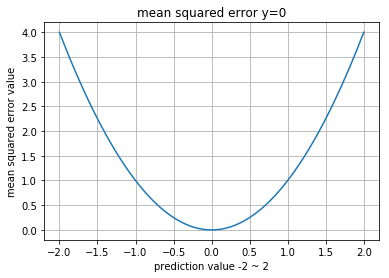
Mean Absolute Error (MAE)
MSE가 large error를 낸다면, MAE의 경우는 상대적으로 작은 에러들을 만듭니다.
하지만 수학적으로 absolute는 많은 연산량을 필요로 합니다.
Numpy
>> def mean_abolute_error(y, p):
>>     return np.abs(y-p).mean()
>>
>> mean_abolute_error(y, p)
0.19
Sklearn
Sklearn 에서는 sklearn.metrics.mean_absolute_error 함수를 사용합니다.
>> metrics.mean_absolute_error(y, p)
0.19
Visualization
>> compare_distributions(mean_abolute_error)
normal_a, normal_a	: 0.0
normal_a, normal_b	: 1.11369204926
normal_a, gumbel  	: 2.57300947501
normal_a, exponent	: 2.13340783974
normal_a, uniform 	: 2.48578624644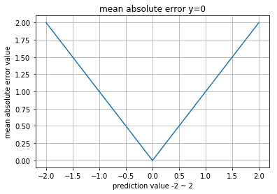
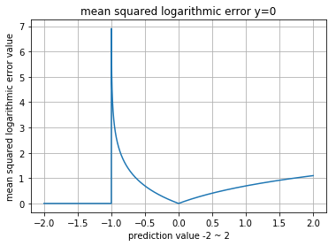
Root Mean Squared Logarithmic Error (RMSLE)
\(p\) 그리고 \(a\) 는 확률.. 즉 0에서 1사이이의 값이 들어가야 합니다.
\[\epsilon = \sqrt{\frac{1}{n} \sum_{i=1}^n (\log(p_i + 1) - \log(a_i+1))^2 }\]Numpy
>> def mean_squared_logarithmic_error(y, p):
>>     try:
>>         l = lambda x: np.nan_to_num(np.log(x + 1))
>>         return np.sqrt(((l(p) - l(y))**2).mean())
>>     except Exception as e:
>>         print(p + 1)
>>         raise e
>>
>> mean_squared_logarithmic_error(y, p)
0.16683918
Visualization
>> compare_distributions(mean_squared_logarithmic_error)
normal_a, normal_a	: 0.0
normal_a, normal_b	: 0.398201741497
normal_a, gumbel  	: 1.40502234456
normal_a, exponent	: 0.890724788695
normal_a, uniform 	: 1.02307079398
0~1사이의 확률 값이 들어가야 하는데, -2 또는 2같은 값이 들어가면서 그래프가 좀 이상하게 보입니다.
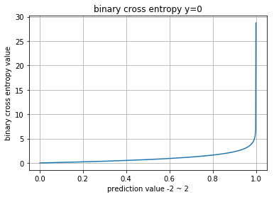
Binary Cross Entropy (a.k.a Logarithmic Loss)
- https://www.kaggle.com/wiki/LogarithmicLoss
Numpy
>> y_true = np.array([0, 0, 0, 1, 0], dtype=np.float64)
>> y_pred = np.array([0.1, 0.1, 0.05, 0.6, 0.3], dtype=np.float64)
>>
>> def binary_cross_entropy(y_true, y_pred):
>>     return -(y_true * np.log(y_pred) + (1-y_true) * np.log(1-y_pred)).mean()
>>
>> binary_cross_entropy(y_true, y_pred)
0.22590297868158524
Sklearn
sklean 에서는 sklearn.metrics.log_loss 함수를 사용합니다.
>> # Scipy와 동일함
>> metrics.log_loss(y_true, y_pred)
0.22590297868158524
Pytorch
F.binary_cross_entropy 와 nn.BCELoss 의 결과값은 동일합니다.
>> y_torch_pred = Variable(torch.DoubleTensor(y_pred))
>> y_torch_true = Variable(torch.DoubleTensor(y_true))
>>
>> torch_crossentropy = nn.BCELoss()
>> torch_crossentropy(y_torch_pred, y_torch_true).data.numpy()
array([ 0.22590298])
Visualization
그래프에서 -2 그리고 2까지 전체 x값이 안나온 이유는 NaN으로 바껴서 해당부분은 안나오는 것입니다.
\(p\) 값은 확률 0~1사이의 값으로 쓰여야 합니다.
Cross Entropy
- https://rdipietro.github.io/friendly-intro-to-cross-entropy-loss/
Partial derivative of the weights
\[\begin{eqnarray} H(y, \hat{y}) &=& -\frac{\partial}{\partial \theta} \sum^N_{i=1} y^{(i)} \log \hat{y}^{(i)} \\ &=& - \sum^N_{i=1} \frac{y^{(i)}}{ \frac{\partial}{\partial \theta} \hat{y}^{(i)}} \\ &=& - \sum^N_{i=1} \frac{y^{(i)}}{ \frac{\partial}{\partial \theta} \left( \theta^{T} \cdot x^{(i)} + b \right) } \\ &=& - \sum^N_{i=1} \frac{y^{(i)}}{x^{(i)}} \end{eqnarray}\]Partial derivative of the bias
\[\begin{eqnarray} H(y, \hat{y}) &=& -\frac{\partial}{\partial b} \sum^N_{i=1} y^{(i)} \log \hat{y}^{(i)} \\ &=& - \sum^N_{i=1} \frac{y^{(i)}}{ \frac{\partial}{\partial b} \hat{y}^{(i)}} \\ &=& - \sum^N_{i=1} \frac{y^{(i)}}{ \frac{\partial}{\partial b} \left( \theta^{T} \cdot x^{(i)} + b \right) } \\ &=& - \sum^N_{i=1} y^{(i)} \end{eqnarray}\]Numpy
>> y_true = np.array([0, 0, 0, 1, 0], dtype=np.float32)
>> y_pred = np.array([0.1, 0.1, 0.05, 0.6, 0.3], dtype=np.float32)
>>
>> def cross_entropy(y_true, y_pred):
>>     return -(y_true * np.log(y_pred)).sum()
>>
>> cross_entropy(y_true, y_pred)
0.51082557
Pytorch - cross entropy
Pytorch의 cross entropy는 일반적인 cross entropy와 전혀 다릅니다.
\[\hat{y}_{class} + \log\left( \sum_j e^{\hat{y}_j} \right)\]>> y_true = np.array([3, 1], dtype=np.int64)
>> y_pred = np.array([[0.1, 0.1, 0.05, 0.6, 0.3],
>> [0, 0.9, 0.05, 0.001, 0.3]], dtype=np.float64)
>>
>>
>> def torch_cross_entropy(y_pred, labels):
>> N = y_pred.shape[0]
>> return (-y_pred[range(N), labels] + np.log(np.sum(np.exp(y_pred), axis=1))).mean()
>>
>> torch_cross_entropy(y_pred, y_true)
1.1437464478328658>> y_true = np.array([3], dtype=np.int64)
>> y_pred = np.array([[0.1, 0.1, 0.05, 0.6, 0.3]], dtype=np.float32)
>>
>> y_torch_true = Variable(torch.LongTensor(y_true))
>> y_torch_pred = Variable(torch.FloatTensor(y_pred))
>>
>> torch_cross_entropy = nn.CrossEntropyLoss()
>> torch_cross_entropy(y_torch_pred, y_torch_true).data.numpy()
array([ 1.26153278], dtype=float32)Pytorch - Custom Cross Entropy
Pytorch에서 제공하는 nn.CrossEntropyLoss는 기존 cross-entropy loss와 다름으로, 정확하게 동일한 코드를 사용시 만들어줘야 합니다.
>> def torch_custom_cross_entropy(y_true, y_pred):
>>     return -torch.sum(y_true * torch.log(y_pred))
>>
>> y_true = np.array([0, 0, 0, 1, 0], dtype=np.float32)
>> y_pred = np.array([0.1, 0.1, 0.05, 0.6, 0.3], dtype=np.float32)
>>
>> y_torch_true = Variable(torch.FloatTensor(y_true))
>> y_torch_pred = Variable(torch.FloatTensor(y_pred))
>>
>> torch_custom_cross_entropy(y_torch_true, y_torch_pred).data.numpy()
array([ 0.51082557], dtype=float32)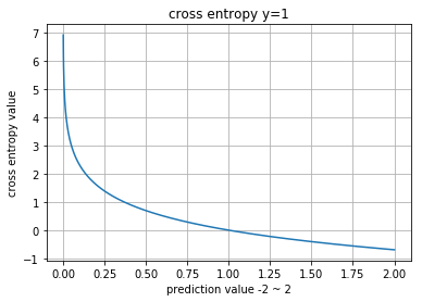
Hinge Loss
logistic과 마찬가지로 binary classification에 사용됩니다.
라이브러리 사용하면 알아서 처리되지만, 기본적으로 labels은 -1 또는 1이어야 합니다.
Numpy
>> p = np.array([0.1, 0.1, 0.05, 0.6, 0.3], dtype=np.float32)
>> y = np.array([-1, -1, -1, 1, -1], dtype=np.float32)
>>
>> def hinge_loss(y, p):
>>     l = 1-(y*p)
>>     l[l<=0] = 0
>>     return l.mean()
>>
>> hinge_loss(y, p)
0.98999995
Sklearn
>> metrics.hinge_loss(y, p)
0.98999999836087227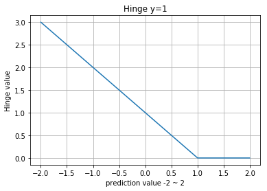
KL-Divergence
\(p\) 그리고 \(q\) 는 확률분포 (0에서 1사이의 값) 이어야 합니다.
\[D_{KL}\left(p(x), q(x)\right) = \sum_{x \in X} p(x) \ln\frac{p(x)}{q(x)}\]참고로.. Scipy.stats.entropy(a, b)를 사용하면 KL-Divergence를 사용하는 것과 마찬가지인데..
내부적으로 nan등 처리가 안되어 있어서 값이 안나옴
Numpy
>> def kl_divergence(y, p):
>>     return np.sum(y * np.nan_to_num(np.log(y/p)), axis=0)
>>
>> compare_distributions(kl_divergence)
normal_a, normal_a	: 0.0
normal_a, normal_b	: 368.575575809
normal_a, gumbel  	: 2596.54562019
normal_a, exponent	: 4806.30679955
normal_a, uniform 	: 6476.72186957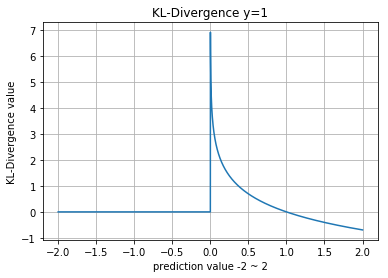
Cosine Proximity
- https://en.wikipedia.org/wiki/Cosine_similarity
Numpy
>> def cosine_proximity(a, b):
>>     norm2 = lambda x: np.sqrt((x**2).sum())
>>     return 1 - (a * b).sum() / (norm2(a) * norm2(b))
>>
>> cosine_proximity(np.array([0.3, 0.4]), np.array([1, 2]))
0.016130089900092459
Visualization
compare_distributions(cosine_distantce)
normal_a, normal_a	: 2.22044604925e-16
normal_a, normal_b	: 0.0998470768358
normal_a, gumbel  	: 0.604350409384
normal_a, exponent	: 0.331605768793
normal_a, uniform 	: 0.188153360738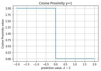
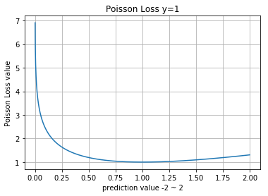
Poisson
- https://github.com/fchollet/keras/pull/479/commits/149d0e8d1871a7864fc2d582d6ce650512de371c
Numpy
>> p = np.array([0.1, 0.1, 0.05, 0.6, 0.3], dtype=np.float32)
>> y = np.array([0, 0, 0, 1, 0], dtype=np.float32)
>>
>> def poisson_loss(y, p):
>>     return (p - y * np.log(p)).mean()
>>
>> poisson_loss(y, p)
0.33216509