Language Modeling - {:.} Installing NLTK - {:.} Word Probability
RNN 101 - {:.} (x_t)는 a vector이고, (x) 는 matrix가 됩니다. - {:.} (s_t = tanh(U_{x_{t}} + W_{s_{t-1}}))
Training Data And PreProcessing - {:.} Tokenize Text - {:.} Initialization - {:.} Forward Propagation - {:.} Predict - {:.} Cross Entropy Loss - {:.} Cross Entropy Loss when y is unknown - {:.} Training the RNN with SGD and Backpropagation Through Time (BPTT) - {:.} Train
Mathmatics behind RNN - {:.} Hyperbolic Tangent - {:.} Softmax Function - {:.} Calculus’ Chain Rule - {:.} RNN Feedworward network
References

Language Modeling

Installing NLTK

sudo pip install numpy
sudo pip install nltk

import nltk
nltk.download('punkt')

Word Probability

이전 문장에 기반하여, 다음 어떤 글자가 올 확률이 높을까? 이런 문제는 다음의 공식을 보면 됩니다.

\[P(w1, ..., w_m) = \prod_{i=1} P(w_i | w_1, ..., w_{i-1})\]

예를 들어서 “In Japan everything is CUTE” 라는 문장의 확률은, “In Japan everything is”라는 단어들이 주어졌을때, CUTE가 올 확률입니다. 즉 $P( \text{"In Japan everything is CUTE"} )$ 의 확률은
$P( \text{CUTE} \ | \ \text{In Japan everything is})$ *
$P( \text{is} \ | \ \text{In Japan everything})$ *
$P( \text{everything} \ | \ \text{In Japan})$ 이렇게 계속 반복..

위 모델링의 문제점은 (Bayes 확률이 그러하듯) 이전의 모든 단어들에 조건이 들어가기 때문에, 너무나 많은 컴퓨팅 파워와 메모리를 요구하며, 이는 현실적으로 거의 불가능한 수준의 모델링입니다. (위의 모델링은 제가 이전에 쓴 Bayes를 이용한 스팸필터링에서도 너무나 많은 컴퓨팅 파워를 요구하기 때문에, Naive Bayes라는 것으로 대체를 하기도 했습니다.) 따라서 현실적으로 위의 공식보다는 RNN을 사용하며, 이론적으로는 RNN은 위의 공식처럼 long-term dependencies를 캡쳐할수 있습니다. (하지만 실제는 RNN또한 앞의 몇 단어정도를 캡쳐하는데 그치며, 제대로 하려면 LSTM이 필요합니다.)

RNN 101

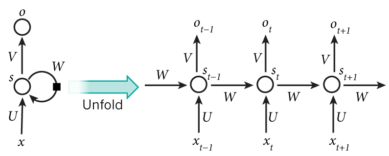
$x_t$는 a vector이고, $x$ 는 matrix가 됩니다.

$s_t = tanh(U_{x_{t}} + W_{s_{t-1}})$

Training Data And PreProcessing

Reddit Comment on Google BigQuery 에서 Reddit Comments를 다운 받을수 있습니다.

Tokenize Text

“He left!” —> “He”, “left”, “!”

일단 Reddit Comments를 다운받으면, Raw text는 있지만, 분석을 위해서는 word단위로 잘라줘야 합니다. 즉 comments를 sentences별로, sentences는 단어 단위로 tokenize가 필요합니다. 이때 punctuation (!)의 경우는 따로 빼줘야 합니다. 예를 들어서 “He left!” 의 경우는 “He”, “left”, “!” 이렇게 빠져야 합니다. Tokenization은 Python NLTK Library의 word_tokenize 그리고 sent_tokenize함수를 통해서 쉽게 해결될수 있습니다.

문장의 처음 시작과, 끝을 알기 위해서 SENTENCE_START, SENTENCE_END를 사용합니다. 또한 RNN에서는 String이 아닌 vectors를 사용하기 때문에 숫자값으로 바꿔줘야 합니다.

[0, 179, 341, 416] –> [179, 341, 416, 255]

0은 SENTENCE_START를 가르키며, 그 다음에 나올 단어를 예측해 나온값이 255이며, 한칸씩 shift해서 결과값에서는 0이 빠져있습니다.

Initialization

SENTENCE_START = 'SETENCE_START'
SENTENCE_END = 'SENTENCE_END'
UNKNOWN_TOKEN = 'UNKNOWN_TOKEN'
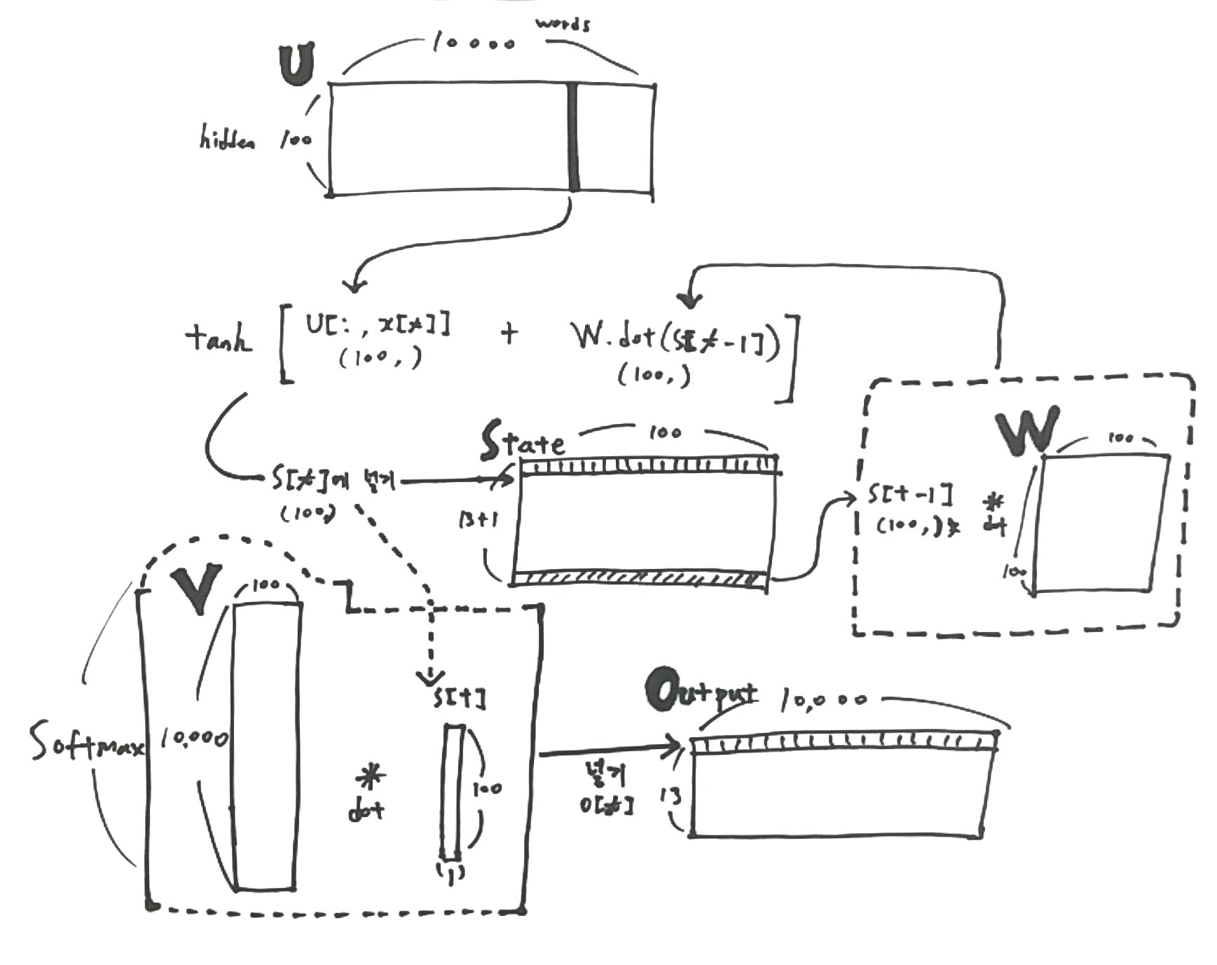
VOCAB_SIZE = 10000

class RNNNumpy(object):
    def __init__(self, word_dim, hidden_dim=100, bptt_truncate=4):
        self.word_dim = word_dim
        self.hidden_dim = hidden_dim
        self.bptt_truncate = bptt_truncate
        self.U = np.random.uniform(-1. / np.sqrt(word_dim), 1. / np.sqrt(word_dim), (hidden_dim, word_dim))
        self.V = np.random.uniform(-1. / np.sqrt(word_dim), 1. / np.sqrt(word_dim), (word_dim, hidden_dim))
        self.W = np.random.uniform(-1. / np.sqrt(word_dim), 1. / np.sqrt(word_dim), (hidden_dim, hidden_dim))

U, V, W를 Initialization을 해줘야 합니다. 여러가지 방법이 있을 수 있지만, 우리는 다음의 공식을 사용해서 초기화를 해줍니다.

\[[ -\frac{1}{\sqrt{n}},\ \frac{1}{\sqrt{n}} ]\]

여기서 n은 previous layer의 connection갯수를 뜻합니다.

Variable	Shape	Python	Description
U	(100, 10000)	self.U.shape	각각의 단어들이 나올수 있는 확률들이 들어있음
V	(10000, 100)	self.V.shape
W	(100, 10000)	self.W.shape

Forward Propagation

def forward_propagation(self, x):
    # The total number of time steps
    T = len(x)
    
    # During forward propagation we save all hidden states in s because need them later.
    # We add one additional element for the initial hidden, which we set to 0
    s = np.zeros((T + 1, self.hidden_dim))

    # The outputs at each time step. Again, we save them for later.
    o = np.zeros((T, self.word_dim))
    for t in xrange(T):
        s[t] = np.tanh(self.U[:, x[t]] + self.W.dot(s[t - 1]))
        o[t] = self.softmax(self.V.dot(s[t]))
    return [o, s]

VOCAB_SIZE = 10000

model = rnn.RNNNumpy(VOCAB_SIZE)
o, s = model.forward_propagation(x_train[9])

예를 들어서 [0, 118, 14, 1603, 7, 92, 9999, 38, 6, 9999, 4787, 2680, 2] 라는 x값이 들어가면, T값은 13이 됩니다.
한 문장을 for문으로 돌면서 output과 state matrix를 연산하게 됩니다.

Variable	Shape	Description
o - output	(13, 10000)	각각의 $o_t$는 전체 vocabulary안에서의 확률을 나태내는 vector
s - state	(14, 100)	문장에서 각각의 단어가 나올수 있는 확률 vector들의 matrix <- U에서 가져옴
s[t - 1]	(100, )	t-1 즉 -1부터 시작하게 되는데, state의 마지막부분에서 시작한다.
U[:, x[t]	(100, )	U에서 특정단어(apple같은..)의 hidden(100)에 속한 모든 확률을 가져옴

Predict

def predict(self, x):
    o, x = self.forward_propagation(x)
    return np.argmax(o, axis=1)
    
p = model.predict(x_train[9])
# [1301 5455 9642 6808 9831 2375 6534 4453 6693 6534 5383 7845  723]

output은 어떤 한 문장이, 전체 vocabulary (10,000개)안에서 나올수 있는 확률의 집합체인데, predict함수는 단순히 이중에서 가장 큰 확률(큰 값)을 argmax로 뽑아낸것..

Cross Entropy Loss

\[L(y, o) = -\sum_{i=0}{ln(o_i) * y_i}\]

예를 들어서 다음과 같은 값이 있다고 한다면..

output         |  y
-------------------------
0.1  0.3  0.6  |  0  0  1
0.2  0.6  0.2  |  0  1  0
0.3  0.4  0.3  |  1  0  0

Squared Error - 첫번째 줄
$(0.1-0)^2 + (0.3-0)^2 + (0.6-1)^2 = 0.01 + 0.09 + 0.16 = 0.26$

Squared Error - 두번째 줄
$(0.2-0)^2 + (0.6-1)^2 + (0.2-0)^2 = 0.04 + 0.16 + 0.04 = 0.24$

Squared Error - 세번째 줄
$(0.3-1)^2 + (0.4-0)^2 + (0.3-0)^2 = 0.49 + 0.16 + 0.09 = 0.74$

따라서 Average mean squared error는 $\frac{(0.26 + 0.24 + 0.74)}{3} = 0.41$

Cross entropy Error - 첫번째 줄
$ln(0.1)*0 + ln(0.3)*0 + ln(0.6)*1 = -(-0.51) = 0.51$

Cross entropy Error - 두번째 줄
$ln(0.2)*0 + ln(0.6)*1 + ln(0.2)*0 = -(-0.51) = 0.51$

Cross entropy Error - 세번째 줄
$ln(0.3)*1 + ln(0.4)*0 + ln(0.3)*0 = -(-1.2) = 1.2$

따라서 Mean cross entropy는 $\frac{(0.51 + 0.51 + 1.2)}{3} = 0.74$

계산식에서 보듯이, Squared Error와 Cross Entropy Error(CE)의 차이점은 CE의 경우 관련 없는 변수들을 0으로 곱해주기 때문에 확률에서 아예 제외를 시켜버립니다. 이런한 특징때문에 classification중에서도 predicting the next word 처럼 엄청나게 많은 분류가 필요한 경우 squared error보다는 cross entropy error가 훨씬더 정확하게 error률을 뽑아냅니다.

Cross Entropy Loss when y is unknown

위의 cross entropy error의 경우 일반적으로 사용하는 경우입니다. 해당의 경우 답이 되는 y의 값을 알고 있는 경우 입니다.
예를 들어서 “I love you”라는 단어에서 output값 (각각의 단어들이 순서대로 나올 확률)과 y 확률이 다음과 같다면..

word | output         |  y
---------------------------------
I    | 0.1  0.3  0.5  |  0  0  1
love | 0.2  0.6  0.2  |  0  1  0
you  | 0.3  0.4  0.3  |  1  0  0

y값의 확률을 알고 있다면.. 무슨 classification처럼.. 그렇다면 위의 공식을 적용할수 있지만,
문제는 다음 단어가 뭐가 올지 우리는 정확한 답을 갖고 있지 않은 상태입니다. 따라서 다른 공식을 사용해야 합니다.

Cross Entropy in Wikipedia 위키피디아를 보면 다음 공식이 있습니다.

\[L(y, o) = - \frac{1}{N} \sum_{i=0}{ln(o_i)}\]

Name	Description
N	전체 text set의 갯수
o - output	어떤 문장에서, 문장의 순서대로 해당 단어가 나올 확률

def cross_entropy(self, x, y):
    N = np.sum((len(sentence) for sentence in y))
    L = 0
    for i in xrange(len(y)):
        o, s = self.forward_propagation(x[i])
        predicted_output = o[np.arange(len(y[i])), y[i]]
        L += np.sum(np.log(predicted_output))
    return -1 * L / N

# model.cross_entropy(x_train[26:27], y_train[26:27])
o.shape: (8, 10000)
s.shape: (9, 100)
x: [[0, 61, 13, 68, 198, 175, 10, 2]]
y: [[61, 13, 68, 198, 175, 10, 2, 1]]
y[i]: [61, 13, 68, 198, 175, 10, 2, 1]
Predicted Output: [.00009  .0001  .00009  .0001  .00009  .00009  .00009  .0001]
cross entropy: 9.21043965588  # 아직 학습이 안되서 매우 높은 상태 :)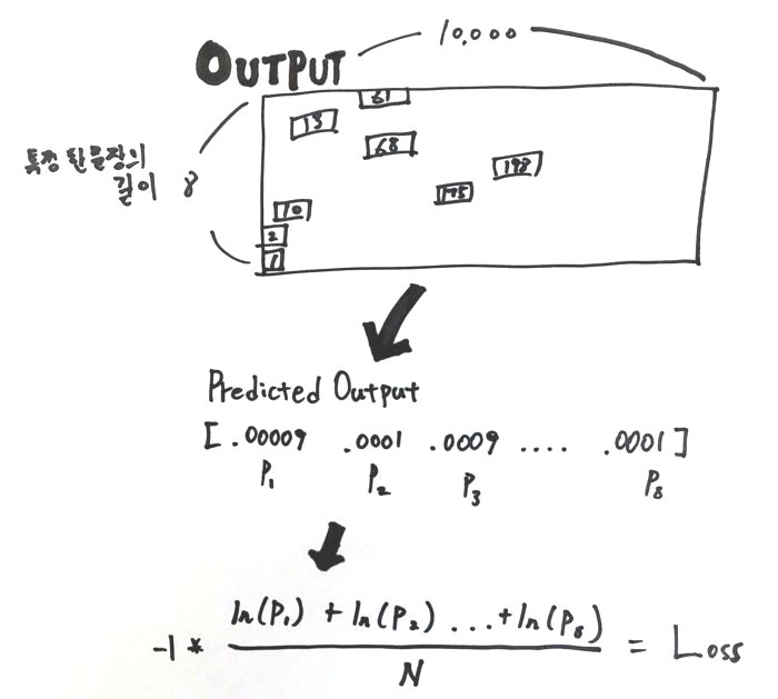

Training the RNN with SGD and Backpropagation Through Time (BPTT)

Training의 궁극적인 목표는 total loss가 가장 적게 나오는 U, V, W값을 알아내는 것 입니다.
일반적으로 Stochastic Gradient Descent(SGD)를 많이 사용합니다.
SGD는 Training Data를 돌면서, error값을 줄이는 방향 그리고 Learning Rate로 U, V, W값들을 조정하는 것입니다.

\[\frac{\partial L}{ \partial U} \ \ \ \frac{\partial L}{ \partial V} \ \ \ \frac{\partial L}{ \partial W}\]

RNN의 경우, 일반적인 Neural Network와는 다르게 time steps을 갖고 있기 때문에, Backpropagation through time (BTPP)를 이용합니다.
일단 SGD는 derivative에 기반하기 때문에 foward, cost error에 사용한 공식들을 정리할 필요가 있습니다.

Example의 forward propagation에서 사용한 공식들

\[s_t = tanh(U x_t + W * s_{t-1})\] \[\hat{y}_t = softmax(V * s_t )\] \[L(y, \hat{y}) = - \frac{1}{N} \sum_{i=0}{ln(\hat{y}_i)}\]

Backpropagation through time

Traditional Neural Network의 경우에는 Backpropagation을 사용하면 되지만, RNN에서는 기존의 약간변형된 BPTT (Backpropagation Through Time) 을 사용합니다. RNN에서는 parameters들이 모든 steps에서 공유가 되기 때문에, gradient를 구할때, 현재의 time step뿐만 아니라 이전의 time steps 까지도 계산이 되어야 합니다. 즉 Calculus의 chain rules 을 사용하면 됩니다.

def bptt(self, x, y):
    """
    :param x: an array of a sentence
    """
    T = len(y)
    o, s = self.forward_propagation(x)
    dldU = np.zeros(self.U.shape)
    dldV = np.zeros(self.V.shape)
    dldW = np.zeros(self.W.shape)
    delta_o = o
    delta_o[np.arange(T), y] -= 1.

    for t in np.arange(T)[::-1]:
        dldV += np.outer(delta_o[t], s[t].T)
        # Initial delta calculation
        delta_t = self.V.T.dot(delta_o[t]) * (1 - (s[t] ** 2))

        for bptt_step in np.arange(max(0, t - self.bptt_truncate), t + 1)[::-1]:
            dldW += np.outer(delta_t, s[bptt_step - 1])
            dldU[:, x[bptt_step]] += delta_t
            delta_t = self.W.T.dot(delta_t) * (1 - s[bptt_step - 1] ** 2)
    return dldU, dldV, dldW

Stochastic Gradient Descent

def calculate_gradients(self, x, y, learning_rate=0.001):
    # Calculate the gradients
    dLdU, dLdV, dLdW = self.bptt(x, y)
    # Change parameters according to gradients and learning rate
    self.U -= learning_rate * dLdU
    self.V -= learning_rate * dLdV
    self.W -= learning_rate * dLdW

Train

def train(self, x_train, y_train, learning_rate=0.005, npoch=100):
    N = len(y_train)
    loss_show = N / 10

    for i in xrange(npoch):
        # One SGD step
        rand_idx = randint(0, N)
        self.calculate_gradients(x_train[rand_idx], y_train[rand_idx], learning_rate)

Mathmatics behind RNN

Hyperbolic Tangent

\[tanh(z) = \frac{sinh(z)}{cosh(z)} = \frac{e^{z} - e^{-z}}{e^{z} + e^{-z}} = \frac{e^{2z} - 1}{ e^{2z} + 1}\]

data = np.arange(-3, 3, 0.1)
plot(data, np.apply_along_axis(np.tanh, axis=0, arr=data))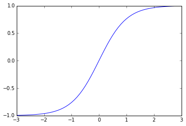

data2 = pd.Series([-1, -0.5, 0, 1, 1.5, 2])
data2.apply(np.tanh)
0   -0.761594
1   -0.462117
2    0.000000
3    0.761594
4    0.905148
5    0.964028
dtype: float64

def tanh(x):
    return np.sinh(x)/np.cosh(x)
data2.apply(tanh)
0   -0.761594
1   -0.462117
2    0.000000
3    0.761594
4    0.905148
5    0.964028
dtype: float64

def tanh2(x):
    return (np.e**(2*x) - 1)/(np.e**(2*x)+ 1)
data2.apply(tanh2)
0   -0.761594
1   -0.462117
2    0.000000
3    0.761594
4    0.905148
5    0.964028
dtype: float64

Softmax Function

\[\frac{exp(x_{i})}{\sum_{j}{exp(x_{j})}}\]

def softmax(x):
    return np.exp(x)/np.sum(np.exp(x))

data = np.arange(-2, 5, 0.1)
plot(data, softmax(data))

[  9.59909960e-05   1.06086457e-04   1.17243667e-04   1.29574291e-04
   1.43201739e-04   1.58262397e-04   1.74906998e-04   1.93302128e-04
   2.13631890e-04   2.36099752e-04   2.60930580e-04   2.88372889e-04
   3.18701330e-04   3.52219442e-04   3.89262684e-04   4.30201797e-04
   4.75446515e-04   5.25449662e-04   5.80711685e-04   6.41785666e-04
   7.09282854e-04   7.83878783e-04   8.66320034e-04   9.57431708e-04
   1.05812568e-03   1.16940973e-03   1.29239762e-03   1.42832027e-03
   1.57853802e-03   1.74455431e-03   1.92803069e-03   2.13080345e-03
   2.35490201e-03   2.60256921e-03   2.87628381e-03   3.17878521e-03
   3.51310097e-03   3.88257703e-03   4.29091122e-03   4.74219029e-03
   5.24093080e-03   5.79212430e-03   6.40128733e-03   7.07451660e-03
   7.81855000e-03   8.64083409e-03   9.54959854e-03   1.05539386e-02
   1.16639060e-02   1.28906097e-02   1.42463270e-02   1.57446262e-02
   1.74005030e-02   1.92305299e-02   2.12530224e-02   2.34882223e-02
   2.59585002e-02   2.86885795e-02   3.17057837e-02   3.50403101e-02
   3.87255317e-02   4.27983314e-02   4.72994712e-02   5.22740000e-02
   5.77717046e-02   6.38476078e-02   7.05625193e-02   7.79836443e-02
   8.61852557e-02   9.52494382e-02]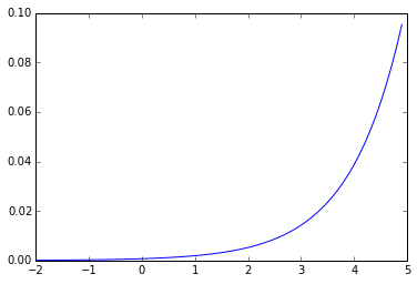

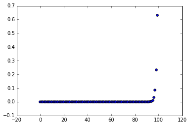
data = np.arange(0, 100, 1)
scatter(data, softmax(data))

그래프에서 보이듯이, 0.1이하로 대부분이 있고, 상위 일부만이 0.1을 넘어서 1에 가까워지는 형태..

Calculus’ Chain Rule

만약 $f(x) = e^{sin(x^2)}$ 라는 공식이 있다면.. 다음과 같이 풀어서 쓸수도 있습니다.

$$ \frac{d{f}}{d{x}} = \frac{df}{du} * \frac{du}{dh} * \frac{dh}{dx} $$

이때 $f(x) = e^x$, $u(x) = sin(x)$, 그리고 $h(x) = x^2$ 이며 f(x)를 풀어서 쓰면 다음과 같습니다.

\[f(u(h(x))) = e^{u(h(x))}\] \[\frac{df}{du} = e^{g(h(x))}, \ \ \frac{du}{dh} = cos(h(x)), \ \ \frac{dh}{dx} = 2x\]

derivative of e^x 는 그냥 e^x
derivative of sin(x) = cos(x)
derivative of x^2 = 2x

따라서 다음과 같은 결론이 날 수 있습니다.

$$ \frac{d{f}}{d{x}} = e^{\sin x^2} * \cos x^2 * 2x $$

RNN Feedworward network

Neural Layer	Description	Index
x(t)	input layer	i
s(t - 1)	previous hidden (state) layer	h
s(t)	hidden (state) layer	j
y(t)	output layer	k

Weight Layer	Description	Index	Code
U	Input layer -> Hidden layer	i, j	U[:, x[t]]
W	Previous hidden layer -> Hidden layer	h, j	W.dot(s[t-1])
V	Hidden layer -> Output layer	j, k	softmax(V.dot(s[t]))

s[t] = np.tanh(self.U[:, x[t]] + self.W.dot(s[t - 1]))

\[net_j(t) = \sum_{i} x_i(t) * U_{ji} + \sum_h W_{jh} * s_h(t-1) + bias_j\] \[\hat{y}_j(t) = f(net_j)\]

o[t] = self.softmax(self.V.dot(s[t]))

\[net_k(t) = \sum_{j} V_{kj} * \hat{y}_j(t) + bias_k\] \[\hat{y}_k(t) = g(net_k)\]

References

WildML - Recurrent Neural Network 에서 거의 대부분의 자료들을 가져왔습니다. 파이썬으로 자세하게 써주셔서 감사합니다.

BPTT 논문에서 BPTT Backpropagation에 관한 내용을 가져왔습니다.

Recurrent Neural Network with Python