Time-Series Decomposition
Introduction
Time series decomposition은 복잡한 시계열 데이터를 각각의 컴포넌트 파트로 쪼개는 과정입니다.
수리적으로 표현하면 다음과 같습니다.
Additive Decomposition
\[y_t = S_t + T_t + C_t + R_t\]Multiplicative Decomposition
\[\begin{align} y_t &= S_t \times T_t \times C_t \times R_t \\ \log y_t &= \log S_t + \log T_t \times \log C_t \times \log R_t \end{align}\]- \(y_t\) : 데이터
- \(S_t\) : Seasonal component
- \(T_t\) : Trend-cycle component
- \(C_t\) : Cyclical component (보통 Cyclical 그리고 Remainder를 합쳐서 Noise 로 보기도 함)
- \(R_t\) : Remainder component
- 이게 무슨 의미?
- 시계열 데이터로 예측할때 component를 나눈후 따로따로 데이터를 취급하여 예측력을 높임
- Additive Decomposition 특징
- 선형 모델링. 변화가 지속적으로 고르게 일어남.
- Multiplicative Decomposition 특징
- 비선형 모델링. Quadratice 또는 exponential 변화가 일어나는 곳에 쓰임.
- 주식은 비선형에 가까움
- 기타
- 두개의 decompositions 을 합쳐서 사용하기도 함
- 현실에서는 그냥 한번에 끝나지 않을수도 있음.
decomposition을 하기전에 많은 데이터 전처리가 들어갈수도 있음
Classical Decomposition
- Seasonal Period
- 분기 데이터:
m = 4(1분기, 2분기,.. 4분기) - 월별 데이터:
m = 12(1월, 2월.. 12월) - 일별 데이터:
m =7(월, 화, … 일)
- 분기 데이터:
Classical decomposition에서는 seasonal period값이 상수값으로 사용합니다.
즉 주가처럼 변화가 심한 것은 다른 알고리즘이 맞음
Additive Decomposition
- Trend Cycle 을 계산
- 공식: \(\hat{T}_t = MA(m)\)
- 원래 공식은 m이 odd 또는 even이냐에 따라 공식이 달라지는데 그냥 MA구한다고 생각하면 됨
- Detrended Series 계산 :
- Detranded Series = \(y_t - \hat{T}_t\)
- Seasonal Component 계산
- 예를 들어 월별 데이터에서 3월의 seasonal 값을 구한다면.. 모든 3월 데이터의 평균값을 구합니다.
- 예) (2019년 3월 + 2020년 3월 + 2021년 3월)/3 = averaged seasonality
- Remainder Component 계산
- 공식: \(R_t = y_t - \hat{T}_t - \hat{S}_t\)
- \(MA(m)\) : Moving average of order m -> MA(4) 면 df.rolling(4).mean() 과 같음
Multiplicative Decomposition
Additive 와 매우 유사합니다.
- MA계산.
- Detrended Series = \(y_t\ / \ \hat{T}_t\)
- Additve decomposition과 동일
- 공식: \(R_t = y_t \big/ \left(\hat{T}_t \times \hat{S}_t \right)\)
의견
- Classical decomposition은 자주 사용되나 추천은 안함. 이유..
- MA를 구하면서 앞, 뒤 데이터가 잘려나감
- Seasnal change에 약함.
예를들어 60년대 전기 사용이 겨울철이 많았다면,
현재는 에어컨 사용으로 여름에 더 전기 사용량이 많음.
-> classical decomposition이 이런 변화에 약함 - 항공 산업 전체에서 일시적인 파업등으로 일부 데이터가 잠시 변화가 있을시.. 여기에 robust하게 대처 못함
Python Code
import pandas as pd
import kaggle.api as kaggle
from tempfile import gettempdir
from pathlib import Path

data_path = Path(gettempdir()) / 'AirPassengers.csv'

kaggle.authenticate()
kaggle.dataset_download_files('rakannimer/air-passengers', data_path.parent, unzip=True)
df = pd.read_csv(data_path, index_col=0)
df.index = pd.to_datetime(df.index)
from statsmodels.tsa.seasonal import seasonal_decompose
# 월별 데이터라서 period=12 로 잡음. 값 안넣어도 자동으로 12로 잡힘
# model="multiplicative" 넣으면 multiplicative decomposition 함
dec = seasonal_decompose(df, model='additive', period=12)
fig = dec.plot()
fig.set_size_inches(9, 5)
Filters
Hodrick Prescott Filter
Data Smoothing technique 으로 주로 사용되며, short-term fluctuations을 제거하는데 사용됩니다.
아래 공식을 보면 T_{t+1} - T_t 부분이 있는데, 미래시점의 데이터를 가져와서 계산을 합니다.
즉 Forecasting 모델에 사용시 해당 필터를 사용시 미래시점의 정보를 이미 input에 갖고 있기 때문에 사용하면 안됩니다.
- \(T_t\) : Trend
- \(C_t\) : Cycle
위의 공식처럼 구성되어 있으며, 최적화하는 방법에 있어서 아래의 Quadratic loss function을 minimize 합니다.
이때 \(\lambda\) 는 smoothing parameter 입니다.
Lambda 는 다음과 같이 사용합니다.
- Quarterly Data (기본값): 1600
- Monthly Data: 129600 ( \(1600 \times 3^4\) )
- Annual Data: 6.25 ( \(1600\ /\ 4^4\) )
from statsmodels.tsa.filters.hp_filter import hpfilter

cycle, trend = hpfilter(air_d, lamb=1600)

# Visualization
fig, ax = plt.subplots(3, 1, figsize=(7, 5))
fig.set_tight_layout(True)
ax[0].plot(air_df)
ax[0].set_title('Price')
ax[1].plot(trend)
ax[1].set_title('Trend')
ax[2].plot(cycle)
ax[2].set_title('Cycle')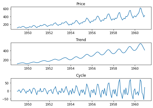
STL Decomposition
STL은 “Seasonal and Trend Decomposition Using Loess”의 약자 이며,
Loess method는 Non-linear 데이터에 사용됩니다.
STL은 기존의 classical decomposition, X11, SEATS 등의 알고리즘보다 좋은 어드벤티지를 갖습니다.
- Advantages
- X11, SEATS등은 특히 monthly, quaterly 에만 사용이 가능하지만,
STL의 경우 모든 타입의 seasonality 데이터에 적용이 가능 - Seasonal component는 시간에 따라 변화하며, 변화량 자체를 유저가 설정 가능
- Trend-Cycle의 smoothness또한 사용자에 의해서 컨트롤이 가능
- Outliers에 robust합니다. 즉 레어한 케이스로 일어나는 급작스러운 변화에 trend-cycle 또는 seasonality에 영향을 주지 않습니다.다만 remainder component에는 영향을 미칩니다.
- X11, SEATS등은 특히 monthly, quaterly 에만 사용이 가능하지만,
- Disadvantages
- 주가의 경우 토요일, 일요일 같은 데이터가 없는데.. 이런 캘린더상의 데이터를 잘 처리하지 못함.
따라서 STL에 넣기전에 그냥 일별 데이터로 전부다 만들어준다음에 넣어야 함
- 주가의 경우 토요일, 일요일 같은 데이터가 없는데.. 이런 캘린더상의 데이터를 잘 처리하지 못함.
Python Code
STL for Air Passengers
from statsmodels.tsa.seasonal import STL

stl = STL(air_df, seasonal=13)
res = stl.fit()
fig = res.plot()
fig.set_size_inches(12, 7)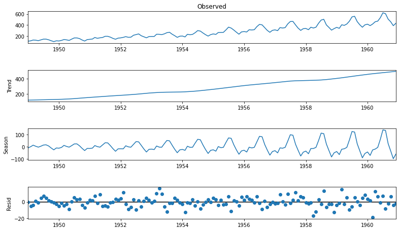
Recompose
Decomposition 으로 시계열 데이터를 분리 했다면.. 다시 합치는 것도 가능.
다만 recompose 시키면서.. 아주 작은 소수점 정도가 틀려 질수 있습니다.
따라서 예측 분야가 아니라.. 아주 정밀한 작업을 요할때는 사용 불가능
stl = STL(air_df, seasonal=13)
res = stl.fit()

# 합치기
recomposed_series = res.trend + res.seasonal + res.resid

# 검증
(recomposed_series.values != air_df.values).sum()
df = pd.DataFrame({'recomposed': recomposed_series, 'air': air_df['#Passengers']})
df['diff'] = df['recomposed'] - df['air']
df[df['diff'] != 0]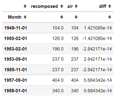
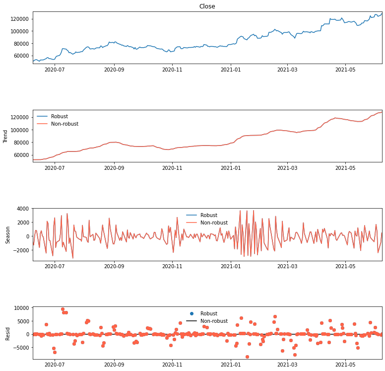
STL Robust Fitting for Stock
- 주가에 robust 옵션이 뭐 그닥
def preprocess(df):
    """
    주가 데이터 전처리
     - 월~금까지 데이터를 남겨두고 지운다.
     - 휴장일의 경우 전날의 데이터를 그대로 사용
     - 이렇게 하는 이유는 5일 로테이션을 맞추기 위해서 (Seasonality)
    """
    df = df.copy()
    datetime_index = pd.DatetimeIndex(pd.date_range(df.index[0], df.index[-1]))

    df = df.reindex(datetime_index)
    df = df.loc[~df.index.weekday.isin({5, 6})]

    df.fillna(method='ffill', inplace=True)
    df.index.name = 'datetime'
    return df

def add_stl_plot(fig, res, legend):
    """Add 3 plots from a second STL fit"""
    axs = fig.get_axes()
    comps = ['trend', 'seasonal', 'resid']
    for ax, comp in zip(axs[1:], comps):
        series = getattr(res, comp)
        if comp == 'resid':
            ax.plot(series, marker='o', linestyle='none', color='tomato')
        else:
            ax.plot(series, color='tomato')

        ax.legend(legend, frameon=False)

df = preprocess(stock)

stl = STL(df.Close, seasonal=5, robust=True)
res = stl.fit()
fig = res.plot()
fig.set_size_inches(12, 12)


add_stl_plot(fig, res, ['Robust', 'Non-robust'])
display(stl.config){'period': 5,
'seasonal': 5,
'seasonal_deg': 1,
'seasonal_jump': 1,
'trend': 11,
'trend_deg': 1,
'trend_jump': 1,
'low_pass': 7,
'low_pass_deg': 1,
'low_pass_jump': 1,
'robust': True}