Deep Residual Neural Network
Deep Residual Learning for Image Recognition
Degradation Problem
Deep convolutional neural networks가 나온 이후로 많은 발전이 있었습니다.
기본적으로 deep networks는 features들을 스스로 low/mid/high level features로 나누며\(^{[01]}\), 근래의 모델들의 경우 layers층을 더 깊이 있게 쌓아서 features들의 levels을 더욱 세분화하고자하는 시도가 있으며\(^{[02]}\), ImageNet 챌린지에서 16개 또는 30개등의 layers를 사용하는 매우 깊은 모델들을 사용하기도 하였습니다.\(^{[03]}\)
단순히 layers를 더 많이 쌓으면 더 좋은 결과를 낼 것인가? 라는 질문에는.. 사실 문제가 있습니다.
이미 잘 알려진 vanishing/exploding gradients\(^{[04]}\) \(^{[05]}\)의 문제는 convergence자체를 못하게 만듭니다.
이러한 문제는 normalized initialization\(^{[06]}\) \(^{[04]}\) \(^{[07]}\), 그리고 intermediate normalization layers \(^{[08]}\)에 의해서 다소 해결이 되어 수십층의 layers들이 SGD를 통해 convergence될 수 있도록 도와줍니다.
Deeper networks를 사용할때 degradation problem이 발견되었습니다. degradation problem은 network의 depth가 커질수록 accuracy는 saturated (마치 뭔가 가득차서 현상태에서 더 진전이 없어져 버리는 상태)가 되고 degradation이 진행됩니다. 이때 degradation은 overfitting에 의해서 생겨나는 것이 아니며, 더 많은 layers를 넣을수록 training error가 더 높아집니다.\(^{[09]}\) (만약 overfitting이었다면 training error는 매우 낮아야 합니다.)
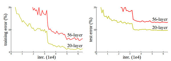
20-layers 그리고 56-layers를 사용했으며, 더 깊은 네트워크일수록 training error가 높으며, 따라서 test error또한 높다.
한가지 실험에서 이를 뒷받침할 근거를 내놓습니다.
shallow network에서 학습된 모델위에 다층의 layers를 추가적으로 쌓습니다. 이론적으로는 deeper 모델이 shallower 모델에 추가된 것이기 때문에 더 낮은 training error를 보여야 합니다. 하지만 학습된 shallower 모델에 layers를 더 추가시켜도, 그냥 shallow 모델보다 더 높은 training error를 보여줍니다.
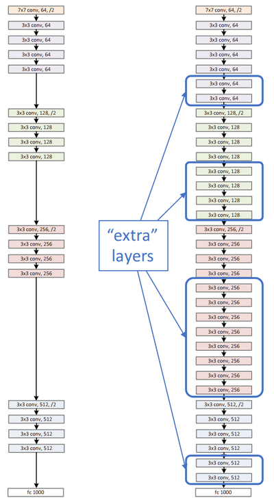
Shallower model(왼쪽) 그리고 Deeper model(오른쪽).
Shallower model로 부터 학습된 지식을 복사하고, Identity mapping로서 layers를 추가하였다.
Deeper model은 shallower model과 비교하여 더 낮거나 같은 training error를 보여야 하지만
실제는 degradation현상으로 인하여 layers가 깊어질수록 training error는 높아진다
위의 그림에서 보듯이, shallower model로 부터 학습된 지식을 복사하고, 추가적으로 identity mapping으로서 layers를 더 추가하였습니다.
여기서 identity mapping이라는 뜻은 \(f(x) = x\) 의 의미로 기존 학습된 layers에서 나온 output을 추가된 layers에서 동일한 output을 생성하는 것입니다. 따라서 identity mapping으로서 추가된 layers들은 최소한 shallower model에서 나온 예측치와 동일하거나 또는 더 깊게 들어갔으니 더 잘 학습이 되어야 합니다.
하지만 현실은.. layers가 깊어지면 깊어질수록 training error가 더 높아지며, 따라서 test error또한 동일하게 높아집니다.
이러한 현상을 degradation problem이라고 하며, Deep Residual Network\(^{[10]}\)가 해결하려는 부분입니다.
Residual
먼저 residual에 대해서 알아야 합니다.
간단하게 이야기 하면 residual이란 관측치(observed data)와 예측값(estimated value)사이의 차이입니다.
Linear least square (최소회귀직선) residual의 합은 0이 됩니다.
예를 들어 다음의 수식에서 true값인 \(x\)를 찾고자 합니다.
이때 $ x $의 근사치(approximation)인 \(x_0\)가 주어졌을때, residual값은 다음과 같습니다.
\[b - f(x_0)\]반면에 error는 true값에서 근사치(approximation)의 차이이며 다음과 같습니다.
(하나의 예로.. 근사값 3.14 - \(\pi\) 가 바로 오차입니다.)
좀더 잘 설명한 영상을 참고 합니다.
ResNet Explained
Degradation에서 언급한 현상을 보면, 직관적으로 보면 deep neural network에 더 많은 layers를 추가시킵으로서 성능을 향상시킬수 있을거 같지만 그와는 정 반대의 결과가 나왔습니다. 이것이 의미하는 바는 multiple nonlinear layers안에서 identity mappings을 시키는데(approximate) 어려움이 있다는 것입니다. 이는 흔히 딥러닝에서 나타나는 vanishing/exploding gradients 이슈 그리고 curse of dimensionality problem등으로 나타나는 현상으로 생각이 됩니다.
ResNets은 이러한 문제를 해결하기 위하여, residual learning을 통해 강제로 Identity mapping (function)을 학습하도록 하였습니다.
- \(x\): 해당 레이어들의 input
- \(H(x)\): (전체가 아닌) 소규모의 다층 레이어(a few stacked layers)의 output
- \(id(x)\): Identity mapping(function)은 단순히 \(id(x) = x\) 으로서, \(x\)값을 받으면 동일한 \(x\)를 리턴시킵니다
- \(H(x)\) 그리고 \(x\) 는 동일한 dimension을 갖고 있다고 가정
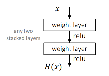
일반적인 Neural Network는 \(H(x)\) 자체를 학습니다.
ResNet의 경우에는 residual function을 학습하도록 강제합니다.
\[F(x) = H(x) - id(x)\]우리는 실제 true값을 알고자 하는 것이기 때문에 위의 공식은 다음과 같이 재정립(reformulation)할수 있습니다.
\[\begin{align} H(x) &= F(x) + id(x) \\ &= F(x) + x \end{align}\]즉 아래의 그림처럼 그래프가 그려집니다.
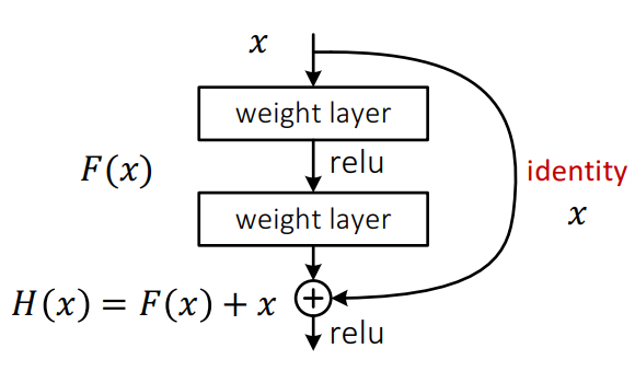
이론적으로 identity mappings이 최적화(optimal)되었다면, 다중 레이어의 weights연산 \(F(x)\) 의 값을 0으로 만들것입니다. \(F(x)\) 가 0이 된후 \(id(x)\) 를 더하기 때문에 해당 subnetwork는 identity function으로서 기능을 하게 됩니다.
실제로는 identity mappings (layers)가 최적화되어 0으로 수렴하는 것은 일어나기 힘듬니다.
다만 reformulation 된 공식안에 identity function이 존재하기 때문에 reference가 될 수 있고, 따라서 neural network가 학습하는데 도움을 줄 수 있습니다.
Shortcut Connection
위에서 이미 언급한 그래프에서 논문에서는 building block을 다음과 같이 정의하고 있습니다.
(공식을 간략하게 하기 위해서 bias에 대한 부분은 의도적으로 누락되어 있습니다. 당연히 실제 구현시에는 필요합니다.)
\(F(x\ |\ W_i)\) 는 학습되야할 residual mapping을 나타내며, \(x\) 그리고 \(y\)는 각각 input 그리고 output을 나타냅니다.
위의 공식은 아주 간략하게 표현하기 위해서 나타낸것이고 2개의 레이어를 사용하는 경우에는 \(F\) 함수에대한 정의가 바뀝니다.
여기서 \(\sigma\)는 ReLU를 가르킵니다. \(F + x\) 는 shortcut connection을 나타내며 element-wise addition을 연산합니다.
해당 addtion 이후! 두번째 nonlinearity를 적용합니다. (즉 ReLU를 addition이후에 적용하면 됨)
\(F + x\) 를 연산할때 중요한점은 dimension이 서로 동일해야 합니다. 만약 서로 dimension이 다르다면 (예를 들어서 input/output의 channels이 서로 다름) linear projection \(W_s\) 를 shorcut connection에 적용시켜서 dimension을 서로 동일하게 만들어줄수 있습니다.
\[y = F(x\ |\ W_i) + W_s x\]Residual function \(F\)는 사실 상당히 유연합니다.즉 \(F\)는 2개, 3개 또는 3개 이상의 다층을 사용하는 것이 가능합니다.
하지만 만약 \(F\)안에 1개의 레이어만 갖고 있다면 linear layer와 동일해지게 됩니다.
따라서 1개만 갖고 있는 \(F\)는 사실상 의미가 없습니다.
또한 \(F\)는 fully-connected layer 또는 convolution같은 다양한 방법으로 모델링을 할 수 있습니다.
TensorFlow Example
CIFAR-10 image classification ResNet model
Create Your Own ResNet
You might want to customize or make your own ResNet.
The following code shows you how to make your own ResNet.
resnet = ResNet(batch=32)
with tf.variable_scope('input_scope'):
    h = resnet.init_block(filter=[7, 7], channel=[3, 32], max_pool=False)

with tf.variable_scope('residual01'):
    h = resnet.max_pool(h, kernel=[2, 2], stride=[2, 2])
    h = resnet.residual_block(h, filter=[3, 3], channel=[32, 32])
    h = resnet.residual_block(h, filter=[3, 3], channel=[32, 32])
    h = resnet.residual_block(h, filter=[3, 3], channel=[32, 32])
    h = resnet.residual_block(h, filter=[3, 3], channel=[32, 32])
    h = resnet.residual_block(h, filter=[3, 3], channel=[32, 32])
    h = resnet.residual_block(h, filter=[3, 3], channel=[32, 32])

with tf.variable_scope('residual02'):
    h = resnet.max_pool(h, kernel=[2, 2], stride=[2, 2])
    h = resnet.residual_block(h, filter=[3, 3], channel=[32, 64])
    h = resnet.residual_block(h, filter=[3, 3], channel=[64, 64])
    h = resnet.residual_block(h, filter=[3, 3], channel=[64, 64])
    h = resnet.residual_block(h, filter=[3, 3], channel=[64, 64])
    h = resnet.residual_block(h, filter=[3, 3], channel=[64, 64])
    h = resnet.residual_block(h, filter=[3, 3], channel=[64, 64])
    h = resnet.residual_block(h, filter=[3, 3], channel=[64, 64])
    h = resnet.residual_block(h, filter=[3, 3], channel=[64, 64])

with tf.variable_scope('residual03'):
    h = resnet.max_pool(h, kernel=[2, 2], stride=[2, 2])
    h = resnet.residual_block(h, filter=[3, 3], channel=[64, 128])
    h = resnet.residual_block(h, filter=[3, 3], channel=[128, 128])
    h = resnet.residual_block(h, filter=[3, 3], channel=[128, 128])
    h = resnet.residual_block(h, filter=[3, 3], channel=[128, 128])
    h = resnet.residual_block(h, filter=[3, 3], channel=[128, 128])
    h = resnet.residual_block(h, filter=[3, 3], channel=[128, 128])
    h = resnet.residual_block(h, filter=[3, 3], channel=[128, 128])

with tf.variable_scope('residual04'):
    h = resnet.max_pool(h, kernel=[2, 2], stride=[2, 2])
    h = resnet.residual_block(h, filter=[3, 3], channel=[128, 256])
    h = resnet.residual_block(h, filter=[3, 3], channel=[256, 256])
    h = resnet.residual_block(h, filter=[3, 3], channel=[256, 256])
    h = resnet.residual_block(h, filter=[3, 3], channel=[256, 256])
    h = resnet.residual_block(h, filter=[3, 3], channel=[256, 256])

with tf.variable_scope('residual05'):
    h = resnet.max_pool(h, kernel=[2, 2], stride=[2, 2])
    h = resnet.residual_block(h, filter=[3, 3], channel=[256, 512])
    h = resnet.residual_block(h, filter=[3, 3], channel=[512, 512])
    h = resnet.residual_block(h, filter=[3, 3], channel=[512, 512])
    h = resnet.residual_block(h, filter=[3, 3], channel=[512, 512])
    h = resnet.residual_block(h, filter=[3, 3], channel=[512, 512])
    h = resnet.residual_block(h, filter=[3, 3], channel=[512, 512])

with tf.variable_scope('fc'):
    h = resnet.avg_pool(h, kernel=[2, 2], stride=[2, 2])
    h = resnet.fc(h)
h # <- Your Network Created